fmdtools.analyze

Package for analyzing simulation results.

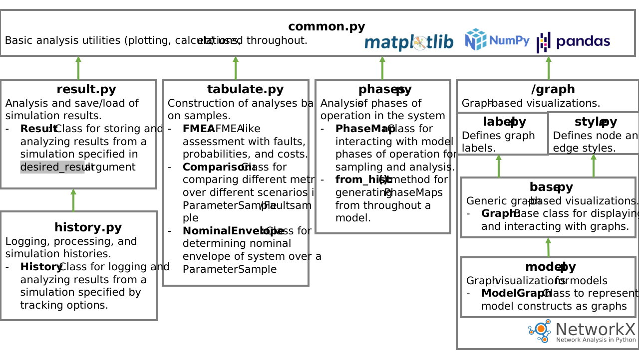
The analyze package is organized into the modules:

fmdtools.analyze.common	Some common methods for analysis used by other modules.
fmdtools.analyze.result	Defines how simulation results (histories) structured and processed.
fmdtools.analyze.history	Defines History: class and for structuring/analyzing simulation histories.
fmdtools.analyze.graph	Package for graph representations and analysis of model structures.
fmdtools.analyze.tabulate	Translates simulation outputs to pandas tables for display, export, etc.
fmdtools.analyze.phases	Module for analyzing phases and time-based sampling schemes.

The model reference for each of these is provided below:

fmdtools.analyze.common

Some common methods for analysis used by other modules.

Has methods:

• bootstrap_confidence_interval(): Convenience wrapper for scipy.bootstrap

• diff(): Helper function for finding inconsistent states between val1, val2, with the difftype option

• join_key(): Helper function for Result Class

• setup_plot(): initializes mpl figure

• plot_err_hist(): Plots a line with a given range of uncertainty around it

• plot_err_lines(): Plots error lines on the given plot

• multiplot_legend_title(): Helper function for multiplot legends and titles

• consolidate_legend(): Creates a single legend for a given multiplot where multiple groups are being compared

• load_folder(): Lists files to load in folder.

• file_check(): Check if files exists and whether to overwrite the file

• auto_filetype(): Helper function that automatically determines the filetype (npz, csv, or json) of a given filename

• create_indiv_filename(): Helper function that creates an individualized name for a file given the general filename and an individual id

fmdtools.analyze.common.add_title_xylabs(ax, title='', xlabel='', ylabel='', zlabel='', xlim=(), ylim=(), zlim=(), aspect='')

Add/set title, x/y labels, and limits to the given axis.

fmdtools.analyze.common.auto_filetype(filename, filetype='', filetypes=['npz', 'csv', 'json'])

Automatically determine the filetype (npz, csv, or json) of a filename.

Examples

>>> auto_filetype("hi.npz")
'npz'
>>> auto_filetype("example.csv")
'csv'
>>> auto_filetype("example.json")
'json'
>>> auto_filetype("x.pdf")
Traceback (most recent call last):
  ...
Exception: Invalid filename in x.pdf, ensure extension is in ['npz', 'csv', 'json'].
>>> auto_filetype("no_ext", "csv")
'csv'

fmdtools.analyze.common.calc_average(data, weights=None, rates=None, **kwargs)

Calculate the average value of given data using calc_metric.

Examples

>>> calc_average([0, 5, 10])
np.float64(5.0)
>>> calc_average([0, 5, 10], [0.0, 0.5, 0.5])
np.float64(7.5)

fmdtools.analyze.common.calc_expected(data, rates=None, weights=None, **kwargs)

Calculate the expected value of given data using calc_metric.

With no explicit rates, use equal probability over the selected axis/axes. Explicit rates retain their existing weighted-sum interpretation.

Examples

>>> calc_expected([0, 5, 10]) # defaults to average
np.float64(5.0)
>>> calc_expected([0, 5, 10], [0.1, 0.5, 0.1])
np.float64(3.5)

fmdtools.analyze.common.calc_metric(data, method=<function average>, args=(), axis=None, dtype=None, rates=None, r_dtype=None, r_norm=False, round_value=True, res=1e-06, min_r=7, **kwargs)

Calculate a metric from data.

Parameters:

• data (array/list/tuple) – Data to take metric over.

• method (method, optional) – Method to call to calculate the metric. The default is np.average.

• args (tuple, optional) – Arguments to the method. The default is ().

• axis (int, optional) – Axis of the array to take the metric over. The default is None.

• dtype (type, optional) – Datatype to pre-process to, if the datat should be interpreted as a different data (e.g., preprocess as bool to calculate a rate). The default is None.

• rate (array/list/tuple, optional) – Array of rates corresponding to data to weight the data by before calculating the metric. The default is None.

• r_dtype (type, optional) – Datatype to preprocess the rates over. The default is None.

• r_norm (bool, optional) – Whether to normalize rates. The default is False.

• round_value (bool, optional) – Whether to round the final value, including named metrics. Applied once after evaluation. Default is True.

• res (float) – Resolution to round to. Default is 1e-6.

• min_r (int) – Maximum number of digits to round to (see round_float).

• **kwargs (kwargs) – Keyword arguments to method (see round_float).

Returns:

metric – Metric calculated by method over data.

Return type:

np.float64/np.int64

Examples

>>> calc_metric([1,2,3]) # simple average
np.float64(2.0)
>>> calc_metric([1,2,3], rates=[0.1, 0.1, 0.0], method=np.sum) # weighted sum
np.float64(0.3)
>>> calc_metric([0, 20, 30], dtype=bool, rates=[0.1, 0.1, 0.1], method=np.sum) # rate of nonzero event
np.float64(0.2)
>>> calc_metric([0, 1, 2], "total")
np.int64(2)
>>> calc_metric([0, 1, 2], "expected", rates=[1.0, 2.0, 1.0])
np.float64(4.0)

fmdtools.analyze.common.calc_metric_ci(data, method=<function average>, return_anyway=False, interval=None, axis=0, **kwargs)

Return bootstrapped confidence interval over calc_metric (or other methods).

Parameters:

• data (data) – data for calc_metric.

• return_anyway (bool, optional) – Whether to return even if the bootstrap cannot be taken (e.g., for plotting). The default is False.

• axis (int) – Axis along which to calculate the confidence interval(s). The default is 0.

• **kwargs (kwargs) – Keyword arguments to the statistic, preprocessing, or scipy.bootstrap. Statistic arguments are used for both the point estimate and resamples.

Returns:

• metric (float) – Metric (e.g., mean)

• ci_low (float) – Lower bound of confidence interval

• ci_high (float) – Upper bound of confidence interval

Examples

>>> calc_metric_ci([[0.0, 0.0, 0.0], [0.0, 0.0, 1.0]], method=np.average)
(array([0. , 0. , 0.5]), array([0., 0., 0.]), array([0., 0., 1.]))
>>> calc_metric_ci([1, 2, 3], method=np.average)
(np.float64(2.0), np.float64(1.0), np.float64(3.0))
>>> calc_metric_ci([[1,2,3], [2,3,4]], method=np.average)
(array([1.5, 2.5, 3.5]), array([1., 2., 3.]), array([2., 3., 4.]))
>>> calc_metric_ci([[1,2,3], [2,3,4]], rates=[0.01, 1.0], method=np.sum)
(array([2.01, 3.02, 4.03]), array([0.02, 0.04, 0.06]), array([4., 6., 8.]))

fmdtools.analyze.common.calc_percent(data, weights=None, rates=None, **kwargs)

Calculate a weighted fraction of non-zero values using calc_metric.

Weights are passed to the averaging method; omitted weights give each value equal influence. Rates remain separate from percentage weights.

Examples

>>> calc_percent([0, 10, 0])
np.float64(0.333333)

fmdtools.analyze.common.calc_rate(data, rates=None, weights=None, **kwargs)

Calculate a rate of a non-zero value in data using calc_metric.

With no explicit rates, use equal probability over the selected axis/axes. Other dimensions, such as history time, do not dilute each reduced rate.

Examples

>>> calc_rate([0, 10, 0]) # defaults to equal rate
np.float64(0.333333)
>>> calc_rate([0, 10, 100], [0.1, 0.1, 0.1]) # provided rates
np.float64(0.2)

fmdtools.analyze.common.calc_sum(data, weights=None, rates=None, **kwargs)

Calculate the average value of given data using calc_metric.

Examples

>>> calc_sum([0, 5, 10.0])
np.float64(15.0)
>>> calc_sum([0, 5, 10.0], [0.0, 0.5, 0.5])
np.float64(15.0)

fmdtools.analyze.common.calc_total(data, weights=None, **kwargs)

Calculate the total number of non-zero values in data using calc_metric.

Examples

>>> calc_total([0, 10, 0])
np.int64(1)
>>> calc_total([0, 10, 100])
np.int64(2)

fmdtools.analyze.common.clear_prev_figure(**kwargs)

Clear previous animations for plot_from methods.

fmdtools.analyze.common.consolidate_legend(ax, loc='upper left', bbox_to_anchor=(1.05, 1), add_handles=[], remove_empty=True, color='', new_labs={}, old_legend=False, **kwargs)

Create a single legend for plots where multiple groups are being compared.

Parameters:

• ax (matplotlib axis) – Axis object to mark on

• loc (str) – Legend location (see matplotlib.legend). Default is ‘upper left’.

• bbox_to_anchor (tuple) – Anchoring bounding box point (see matplotlib.legend). Default is (1.05, 1).

• add_handles (list) – Labelled plot handles to add to the legend. Default is [].

• remove_empty (bool) – If add_handles is used, this toggles whether to add unlabeled entries to the legend. Default is False.

fmdtools.analyze.common.create_indiv_filename(filename, indiv_id, splitchar='_')

Create filename name for a file given general filename and individual id.

Examples

>>> create_indiv_filename("hi.csv", "4")
'hi_4.csv'
>>> create_indiv_filename("runs.v1/results.v2.csv", "4", splitchar="/")
'runs.v1/results.v2/4.csv'

fmdtools.analyze.common.diff(val1, val2, difftype='bool')

Find inconsistent states between val1, val2.

The difftype option (‘diff’ (takes the difference), ‘bool’ (checks if the same),

and float (checks if under the provided tolerance))

Integer arithmetic is widened before subtraction and absolute value. Numeric differences use int64 where possible, or exact Python integers for values outside its range. Boolean comparisons and floating arithmetic are unchanged.

Examples

>>> diff([1, 2, 3], [2, 2, 3])
array([ True, False, False])
>>> diff([1, 2, 3], [2, 2, 3], difftype="diff")
array([-1,  0,  0])

fmdtools.analyze.common.file_check(filename, overwrite)

Check if files exists and whether to overwrite the file.

fmdtools.analyze.common.get_sub_include(att, to_include)

Determine attributes of att to include based on provided dict/str/list/set.

fmdtools.analyze.common.join_key(k)

Join list of keys into single key separated by a ‘.’.

Examples

>>> join_key(["key", "subkey"])
'key.subkey'
>>> join_key("existing_key")
'existing_key'

fmdtools.analyze.common.load_folder(folder, filetype)

Create list of files to be read from a folder.

(e.g., that have been saved from multi-scenario propagate methods with ‘indiv’:True)

Parameters:

• folder (str) – Name of the folder. Must be in the current directory

• filetype (str) – Type of files in the folder (‘npz’, ‘csv’, or ‘json’). Other extensions and subdirectories are ignored; matching files are not searched recursively.

Returns:

files_to_read – files to load for results/mdlhists.

Return type:

list

fmdtools.analyze.common.mark_times(ax, tick, time, *plot_values, fontsize=8, rounddec=1, pretext='t=')

Mark times on an axis at a particular tick interval.

Parameters:

• ax (matplotlib axis) – Axis object to mark on

• tick (float) – Tick frequency.

• time (np.array) – Time vector.

• *plot_values (np.array) – x,y,z vectors

• fontsize (int, optional) – Size of the font. The default is 8.

fmdtools.analyze.common.metric_preamble(data, dtype=None, rates=None, r_dtype=None, r_norm=False)

Process data for weighted metrics used by calc_metric and calc_metric_ci.

Integer and boolean rate factors are promoted to float64 before normalization or multiplication, avoiding fixed-width overflow in risk calculations. Unweighted data and floating/object rate arithmetic are unchanged.

fmdtools.analyze.common.multiplot_helper(cols, *plot_values, figsize='default', titles={}, sharex=True, sharey=False, fig=None, axs=None)

Create multiple plot axes for plotting.

fmdtools.analyze.common.multiplot_legend_title(groupmetrics, axs, ax, legend_loc=False, title='', v_padding=None, h_padding=None, title_padding=0.0, legend_title=None, **kwargs)

Create multiplot legends and titles on shared axes.

fmdtools.analyze.common.phase_overlay(ax, phasemap, label_phases=True)

Overlay phasemap information on plot.

fmdtools.analyze.common.plot_err_hist(err_hist, ax=None, fig=None, figsize=(6, 4), boundtype='fill', boundcolor='gray', boundlinestyle='--', fillalpha=0.3, time='time', xlabel='time', ylabel='', title='', xlim=(), ylim=(), **kwargs)

Plot a line with a given range of uncertainty around it.

Parameters:

• err_hist (History) –

  hist of line, low, high values. Has the form ::

  {‘time’: times, ‘stat’: stat_values, ‘low’: low_values, ‘high’: high_values}

• ax (mpl axis (optional)) – axis to plot the line on

• fig (mpl figure (optional)) – figure to plot line on

• figsize (tuple) – figure size (optional)

• boundtype ('fill' or 'line') – Whether the bounds should be marked with lines or a fill

• boundcolor (str, optional) – Color for bound fill The default is ‘gray’.

• boundlinestyle (str, optional) – linestyle for bound lines (if any). The default is ‘–‘.

• fillalpha (float, optional) – Alpha for fill. The default is 0.3.

• time (str, optional) – history to use as time. The default is ‘time’.

• **kwargs (kwargs) – kwargs for the line

Returns:

• fig (mpl figure)

• ax (mpl, axis)

fmdtools.analyze.common.plot_err_lines(times, lows, highs, ax=None, fig=None, figsize=(6, 4), **kwargs)

Plot error lines on the given plot.

Parameters:

• times (list/array) – x data (time, typically)

• line (list/array) – y center data to plot

• lows (list/array) – y lower bound to plot

• highs (list/array) – y upper bound to plot

• **kwargs (kwargs) – kwargs for the line

fmdtools.analyze.common.prep_animation_title(time, title='', **kwargs)

Add time to titles for plot_from methods.

fmdtools.analyze.common.set_empty_multiplots(axs, num_plots, cols, xlab_ang=-90, grid=False, set_above=True)

Align empty axes with the rest of the multiplot.

fmdtools.analyze.common.setup_plot(fig=None, ax=None, z=False, figsize=(6, 4))

Initialize a 2d or 3d figure at a given size.

If there is a pre-existing figure or axis, uses that instead.

fmdtools.analyze.common.suite_for_plots(testclass, plottests=False)

Qualitative testing suite with or without plots in unittest.

Plot tests should have “plot” in the title of their method, this enables this function tofilter them out (or include them).

Parameters:

• testclass (unittest.TestCase) – Test-case to create the suite for.

• plottests (bool/list, optional) – Whether to show the plot tests (True) or the non-plot tests (False). If a list is provided, only tests provided in the list will be run.

Returns:

suite – Test Suite to run with unittest.TextTestRunner() using runner.run (e.g., runner = unittest.TextTestRunner(); runner.run(suite_for_plots(UnitTests, plottests=False)))

Return type:

unittest.TestSuite

fmdtools.analyze.common.to_include_keys(to_include)

Determine dict keys to include from Result given nested to_include dictionary.

Examples

>>> to_include_keys({"a":{"b": "c"}})
('a.b.c',)
>>> ks = to_include_keys({"a":{"b": {"c", "d", "e"}}})
>>> all([k in ks for k in ('a.b.c', 'a.b.e', 'a.b.d')])
True
>>> to_include_keys("hi")
('hi',)
>>> to_include_keys(["a", "b", "c"])
('a', 'b', 'c')

fmdtools.analyze.common.unpack_plot_values(plot_values)

Upack plot_values if provided as a dict or str.

fmdtools.analyze.result

Defines how simulation results (histories) structured and processed.

Has classes:

• Result: Class for defining simulation results

And functions:

• load(): Loads a given file to a Result/History

Private Methods:

• clean_resultdict_keys(): Helper function for recreating results dictionary keys (tuples) from a dictionary loaded from a file (where keys are strings) (used in csv/json results)

• get_dict_attr(): Gets attributes *attr from a given nested dict dict_in of class des_class

• fromdict(): Creates new history/result from given dictionary

• check_include_errors(): Helper function for Result Class, Cycles through check_include_error

• check_include_error(): Helper function to raise exceptions for errors

• get_sub_include(): Determines what attributes of att to include based on the provided dict/str/list/set to_include

class fmdtools.analyze.result.Result(mapping=None, **kwargs)

Bases: UserDict

Result is a special type of dictionary for simulation results.

The goal of the Result class is to make it convenient to store, access, and load results form a model/simulation. As a dictionary, it supports dict-based item assignment (e.g. r[‘x’]=10) but also enables convenient access via __getattr__, e.g.,:

>>> r = Result()
>>> r['x'] = 10
>>> r
x:                                    10

It also can return a flattened version of its nested structure via Result.flatten(), e.g.,:

>>> r = Result(y=Result(z=1))
>>> r
y:
--z:                                   1
>>> r.keys()
dict_keys(['y'])
>>> rf = r.flatten()
>>> rf
y.z:                                   1
>>> rf['y.z']
1
>>> rf.keys()
dict_keys(['y.z'])
>>> Result({'a': 'b', 'c': {'d': 'e'}})
a:                                     b
c:
--d:                                   e

It also enables saving and loading to files via r.save(), r.load(), and r.load_folder()

align_external_dict(ext_dict)

Align external dict with the order of the Result.

Examples

>>> r = Result({'t1.a': 0.5, 't1.b': 0.01, 't2.a': 0.0, 't2.b': 0.1})
>>> r.align_external_dict({'t2': 1, 't1': 2})
{'t1': 2, 't2': 1}

all()

all_with(attr)

Get all values with the attribute attr.

as_table()

Create a table corresponding to the current dict structure.

create_simple_fmea(*metrics)

Make a simple FMEA-stype table of the metrics in the end-state classification of a list of fault scenarios run. If metrics not provided, returns all

flatten(newhist=False, prevname='', to_include='all')

Recursively create a flattened result of the given nested model history.

Parameters:

• newhist (bool, default = False)

• prevname (tuple, optional) – Current key of the flattened history (used when called recursively). The default is ().

• to_include (str/list/dict, optional) –

  What attributes to include in the dict. The default is ‘all’. Can be of form - list e.g. [‘att1’, ‘att2’, ‘att3’] to include the given attributes - dict e.g. fxnflowvals {‘flow1’:[‘att1’, ‘att2’],

  ’fxn1’:’all’, ‘fxn2’:[‘comp1’:all, ‘comp2’:[‘att1’]]}

  • str e.g. ‘att1’ for attribute 1 or ‘all’ for all attributes

Returns:

newhist – Flattened model history of form: {(fxnflow, …, attname):array(att)}

Return type:

dict

classmethod fromdict(inputdict)

Set up new Result from dictionary.

Examples

>>> d = Result.fromdict({'a': 2, 'b': {'c': 4}})
>>> d
a:                                     2
b:
--c:                                   4
>>> d.b
c:                                     4

get(*argstr, default={}, **to_include)

Provide dict-like access to the history/result across a number of arguments.

Parameters:

• *argstr (str) – keys to get directly (e.g. ‘fxns.fxnname’)

• default (dict or value) – default(s) to use if not in Result. May be a dict of keys {‘k’: val} or a default for all values to get. Default is {}.

• **to_include (dict/str/) – to_include dict for arguments to get (e.g., {‘fxns’:{‘fxnname’}})

Returns:

Result/History with the attributes (or single att)

Return type:

Result/History

Examples

>>> r=Result({'a': 'b', 'c': {'d': 'e'}})
>>> r.get('a')
'b'
>>> r.get('c')
d:                                     e
>>> r.get('c.d')
'e'

get_comp_groups(*values, time='time', **groups)

Get comparison groups of *values (i.e., aspects of the model) in groups **groups (sets of scenarios with structure )

Parameters:

• *values (str) – Values to get (e.g. fxns.fxnname.s.val)

• **groups (list) – Sets of scenarios to group (e.g. set_1=[‘scen1’, ‘scen2’…]). Scenario names match at dot-separated path boundaries; selecting a parent scenario also includes its nested scenarios. Flattened, nested and mixed result storage produce the same groups of leaf paths.

Returns:

group_hist – Single-level history with structure {group:{scenname.valuename}}

Return type:

History

get_default_comp_groups()

Get nominal and faulty keys for single or nested scenario samples.

Nested samples retain their parent prefix (e.g., sample.nominal). Only a scenario named exactly nominal belongs to the nominal group.

Returns:

comp_groups – Dict with structure {‘nominal’: [list of nominal scenarios], ‘faulty’: [list of faulty scenarios]}. If no nominal scenario is found, returns {‘default’: ‘default’}.

Return type:

dict

get_different(other)

Find the values of two results which are different.

Array-valued entries are retained when any element of their difference is nonzero; the full difference array is returned.

Parameters:

other (Result) – Result to compare against

Returns:

different – Result with entries corresponding to the difference between the two Results.

Return type:

Result

get_expected(app=[], with_nominal=False, difference_from_nominal=False, round_value=True, res=1e-06, **kwargs)

Take the expectation of numeric metrics in the result over given scenarios.

Without a nominal scenario, use the first scenario’s numeric fields. A nominal reference is required only for differences from nominal. An empty result returns an empty result of the same type.

Parameters:

• app (SampleApproach, optional) – Approach to use for weights (via rates). The default is [].

• with_nominal (bool, optional) – Whether to include the scenario named exactly ‘nominal’ in the expectation. Other names containing ‘nominal’ remain included. The default is False.

• difference_from_nominal (bool, optional) – Whether to calculated the difference of the expectation from nominal. The default is False.

• **kwargs – kwargs to round_float

Returns:

expres – Result/History with values corresponding to the expectation of its quantities over the contained scenarios.

Return type:

Result/History

get_faulty()

Get fault scenarios without interpreting their names as access aliases.

A single scenario loses its prefix, while multiple scenarios retain theirs. A scenario named ‘faulty’ is selected without recursive lookup.

get_memory()

Determine the memory usage of a given history and profiles.

Returns:

• mem_total (int) – Total memory usage of the history (in bytes)

• mem_profile (dict) – Memory usage of each construct of the model history (in bytes)

get_metric(value, method=<function average>, rates=None, weights=None, prefix='', **kwargs)

Calculate a statistic of the value using a provided metric function.

Parameters:

• value (str) – Value of the history to calculate the statistic over

• weights (str/array) – Keys to use for weights, if any. Default is None.

• rates (str/array) – Keys to use for rates, if any. Default is None.

• prefix (str) – Prefix to get values from. Default is “”.

• **kwargs (kwargs) – Keyword arguments for calc_metric.

Examples

>>> r = Result({'t1.a': 0.5, 't1.b': 0.01, 't2.a': 0.0, 't2.b': 0.1})
>>> r.get_metric("a", method=np.average, rates="b")
np.float64(0.0025)
>>> r.get_metric("a", method="total")
np.int64(1)
>>> r.get_metric("b", method="rate", rates="a")
np.float64(0.5)
>>> r.get_metric("b", method="expected", rates="a")
np.float64(0.005)
>>> r.get_metric("b", "expected", rates={"t1": 1, "t2": 2})
np.float64(0.21)

get_metric_ci(value, method=<function average>, prefix='.', rates=None, weights=None, **kwargs)

Get the confidence interval for the given value over the set of scenarios.

Parameters:

• value (str) – Value of the history to calculate the statistic over

• **kwargs (kwargs) – kwargs to calc_metric_ci

Returns:

• statistic (number) – nominal statistic for the given metric

• lower bound (number) – lower bound of the statistic in the ci

• upper bound (number) – upper bound of the statistic in the ci

Examples

>>> r = Result({'a.a': 1, 'b.a': 3, "c.a": 2})
>>> r.get_metric_ci("a")
(np.float64(2.0), np.float64(1.0), np.float64(3.0))
>>> r.get_metric_ci("a", rates=[0.5, 1.0, 0.5], r_norm=True, method=np.sum)
(np.float64(2.25), np.float64(1.0), np.float64(4.5))

get_metrics(*values, prefix='.', **kwargs)

Calculate a statistic of the values using a provided metric function.

Parameters:

• *values (strs) – Values of the history to calculate the statistic over (if none provided, creates metric of all)

• **kwargs (kwargs) – Keyword arguments to get_metric.

get_scens(*scens)

Get a dictlike with all scenarios corresponding to the strings in *scens.

get_vals(*values, prefix='', **val_kwargs)

Get *values from the dict and return as tuples.

Named keyword values are paired with the first value by their shared path prefix; missing counterparts raise KeyError. External mappings follow the selected scenarios. Explicit arrays retain the caller’s supplied order.

Examples

>>> r = Result({'a': 1, 'b': 3})
>>> r.get_vals("a", c="b")
([1], [3])
>>> r = Result({'x.a': 1, 'y.a': 3})
>>> r.get_vals('a', c={'x': 4, 'y': 5})
([1, 3], [4, 5])

get_values(*values, prefix='')

Select values by complete trailing attribute paths.

Prefix and value are combined before matching. A leading dot requires a nested path; an empty selector retains all values. Partial component suffixes do not match, so x does not select xx or cost select totalcost.

is_flat()

Check if the history is flat.

Examples

>>> Result({'a': 'b', 'c': {'d': 'e'}}).is_flat()
False
>>> Result({'a': 'b', 'c.d': 'e'}).is_flat()
True

items()

Get items iterator (not nested).

keys()

Get keys iterator (not nested).

load(filetype='', renest_dict=False, indiv=False)

Load as Result using :func:`load’.

load_folder(filetype, renest_dict=False)

Load as History using :func:`load_folder’.

nest(levels=inf, separator='.', skip=0)

Re-nest a flattened result.

plot_metric_dist(*values, cols=2, comp_groups={}, bins=10, metric_bins={}, legend_loc=-1, xlabels={}, ylabel='count', title='', titles={}, figsize='default', v_padding=0.4, h_padding=0.05, title_padding=0.1, legend_title=None, indiv_kwargs={}, fig=None, axs=None, **kwargs)

Plot histogram of given metric(s) over comparison groups of scenarios.

Parameters:

• *values (str) – names of values to pull from the result (e.g., ‘fxns.move_water.s.flowrate’) Can also be specified as a dict (e.g. {‘fxns’:’move_water’}) to get all keys from a given fxn/flow/mode/etc.

• cols (int, optional) – columns to use in the figure. The default is 2.

• comp_groups (dict, optional) –

  Dictionary for comparison groups (if more than one). Has structure:

  {'group1': ('scen1', 'scen2'), 'group2': ('scen3', 'scen4')}.
  

  Default is {}, which compares nominal and faulty. If {‘default’: ‘default’} is passed, all scenarios will be put in one group. If a legend is shown, group names are used as labels.

• bins (int) – Number of bins to use (for all plots). Default is None

• metric_bins (dict,) –

  Dictionary of number of bins to use for each metric. Has structure:

  {'metric':num}.
  

  Default is {}

• legend_loc (int, optional) – Specifies the plot to place the legend on, if runs are being compared. Default is -1 (the last plot) To remove the legend, give a value of False

• xlabels (dict, optional) –

  Label for the x-axes. Has structure:

  {'metric':'label'}
  

• ylabel (str, optional) – Label for the y-axes. Default is ‘time’

• title (str, optional) – overall title for the plot. Default is ‘’

• indiv_kwargs (dict, optional) –

  dict of kwargs to differentiate the comparison groups. Has structure:

  {comp1: kwargs1, comp2: kwargs2}
  

  where kwargs is an individual dict of keyword arguments for the comparison group comp (or scenario, if not aggregated) which overrides the global kwargs (or default behavior).

• figsize (tuple (float,float)) – x-y size for the figure. The default is ‘default’, which dymanically gives 3 for each column and 2 for each row

• v_padding (float) – vertical padding between subplots as a fraction of axis height.

• h_padding (float) – horizontal padding between subplots as a fraction of axis width.

• title_padding (float) – padding for title as a fraction of figure height.

• legend_title (str, optional) – title for the legend. Default is None.

• fig (matplotib figure) – Pre-existing figure (if any).

• axs (matplotlib axes) – Pre-existing axes (if any).

• **kwargs (kwargs) – keyword arguments to mpl.hist e.g. bins, etc.

save(filename, filetype='', overwrite=False, result_id='')

Save a given result variable (result or history) to a file filename.

Files can be saved as npz, csv, or json. JSON converts arrays to nested lists of Python values (or a scalar for zero-dimensional arrays). Array dtype and shape metadata are not stored in JSON.

Parameters:

• filename (str) – File name for the file. Can be nested in a folder if desired.

• filetype (str, optional) – Format to write, overriding the filename extension when supplied. The default “” infers the format from the extension. The exact filename is used for all formats; no extension is appended.

• overwrite (bool, optional) – Whether to overwrite existing files with this name. The default is False.

• result_id (str, optional) – For individual results saving. Places an identifier for the result in the file. The default is ‘’.

state_probabilities(prob_key='prob', class_key='classification', prefix='.')

Tabulates the probabilities of different classifications in the result.

Parameters:

• prob_key (str, optional) – string to use for rate/probability information. default is ‘prob’

• class_key (str, optional) – string to use for the different classifications. default is ‘classification’

Returns:

probabilities – Dictionary of probabilities of different simulation classifications

Return type:

dict

total(metric, prefix='.')

Tabulates the total (non-weighted sum) of a metric over a number of runs.

Parameters:

metric (str) – metric to total

Returns:

totalcost – The total metric of the scenarios.

Return type:

Float

values()

Get values iterato (not nested)r.

fmdtools.analyze.result.check_include_error(result, to_include)

Throw error if key not in keys.

fmdtools.analyze.result.check_include_errors(result, to_include)

Throw error if any keys aren’t in the result.

fmdtools.analyze.result.clean_resultdict_keys(resultdict_dirty)

Clean the keys of a loaded dictionary.

Helper function for recreating results dictionary keys (tuples) from a dictionary loaded from a file (where keys are strings) (used in csv/json results).

Parameters:

resultdict_dirty (dict) – Results dictionary where keys are strings

Returns:

resultdict – Results dictionary where keys are tuples

Return type:

dict

fmdtools.analyze.result.clean_to_return(to_return)

Clean the to_return dictionary.

fmdtools.analyze.result.fromdict(resultclass, inputdict)

Create new history/result from given dictionary.

fmdtools.analyze.result.get_dict_attr(dict_in, des_class, *attr)

Get attributes *attr from a given nested dict dict_in of class des_class.

fmdtools.analyze.result.load(filename, filetype='', renest_dict=True, indiv=False, Rclass=<class 'fmdtools.analyze.result.Result'>)

Load a given (result or history) results dictionary from a (npz/csv/json) file.

e.g. a file saved using process.save_result or save_args in propagate functions.

Parameters:

• filename (str) – Name of the file.

• filetype (str, optional) – Use to specify a filetype for the file (if not included in the filename). The default is “”.

• renest_dict (bool, optional) – Whether to return . The default is True.

• indiv (bool, optional) – Whether the result is an individual file (e.g., in a folder of results for a given simulation). The default is False.

• Rclass (class) – Class to return (Result, History, or Dict)

Returns:

result – Corresponding result/hist object with data loaded from the file.

Return type:

Result/History

fmdtools.analyze.result.load_csv(filename, indiv=False)

Load csv files.

fmdtools.analyze.result.load_json(filename, indiv=False)

Load json files.

fmdtools.analyze.history

Defines History: class and for structuring/analyzing simulation histories.

• History: Class for defining simulation histories (nested dictionaries of arrays or lists)

And functions/methods:

• init_dicthist(): Initializes histories for dictionary attributes (if any)

• def prep_hists(): Prepare the history for plotting.

class fmdtools.analyze.history.History(mapping=None, **kwargs)

Bases: Result

Class for recording and analyzing simulation histories.

Histories log states of the model over time.

It can be updated over time t using h.log(obj, t), where obj is an object with (nested) attributes that match the keys of the (nested) dictionary.

Examples

# histories act the same as results, but with the values being arrays:

>>> hist = History({"a": [1, 2, 3], "b": [4, 5, 6], "time": [0, 1, 2]})
>>> hist
a:                              array(3)
b:                              array(3)
time:                           array(3)

history access is the same as a result:

>>> hist.a
[1, 2, 3]

metrics can be gotten from histories over time:

>>> hist = History({"a.a": [1, 2, 3], "b.a": [4, 5, 6], "time": [0, 1, 2]})
>>> hist.get_metric("a", axis=0)
array([2.5, 3.5, 4.5])

or over all times:

>>> hist.get_metric("a")
np.float64(3.5)

animate(plot_func, times='all', figsize=(6, 4), z=False, **kwargs)

Create an animation of a plotting function over the history.

Parameters:

• plot_func (method or str) – External update function for plot. If str, name of internal update method. (e.g., ‘plot_trajectories_from’).

• times (list or all, optional) – Times to animate over. The default is ‘all’.

• figsize (tuple, optional) – Size of the figure. The default is (6, 4).

• z (int/Float/Bool, optional) – Whether to instantiate a z-value. The default is False.

• **kwargs (kwargs) – Keyword arguments.

Returns:

ani – Object with animation.

Return type:

animation.Funcanimation

copy()

Create an independent copy, including mutable objects in array entries.

Non-History entries retain the existing conversion to NumPy arrays.

cut(end_ind=None, start_ind=None, newcopy=False, reshape_to=None)

Cut the history to a given index.

Parameters:

• end_ind (int, optional) – the index of the array that you want to cut the history up to. Default is None.

• start_ind (int, optional) – the index of the array that you want to start cutting the history from. The default is None, which starts from the 0th index.

• newcopy (bool, optional) – Tells whether to creat a new history variable with the information what was cut or cut the original history variable. Default is False.

• reshape_to (int, optional) – Size of array to cut from, if different from current size. Default is None, which does not reshape the array.

Examples

>>> hist = History({'a':[2,3,4,5], 'b':[5,4,3,2,1,0], 'time': [0,1,2,3,4,5]})
>>> cut_hist = hist.cut(3)
>>> cut_hist
a:                              array(4)
b:                              array(4)
time:                           array(4)

>>> cut_hist.a
[2, 3, 4, 5]
>>> cut_hist.b
[5, 4, 3, 2]
>>> cut_hist.time
[0, 1, 2, 3]

classmethod fromdict(inputdict)

Create history from dictionary. Used in initialization.

get_degraded_hist(*attrs, nomhist={}, operator=<function any>, difftype='bool', withtime=True, withtotal=True)

Get history of times when the attributes *attrs deviate from nominal values.

Align the comparison on local flattened views without truncating either source history. Returned values use the common time range.

Parameters:

• *attrs (names of attributes) – Names or dot-separated paths to check (e.g., flow_1, fxn_2). Matches complete path components and their descendants, so pump does not select pump2.

• nomhist (History, optional) – Nominal history to compare against (otherwise uses internal nomhist, if available)

• operator (function) – Method of combining multiple degraded values. The default is np.any. For unlike state shapes, reduce each state at each timestamp before combining states, preserving the time axis.

• difftype ('bool'/'diff'/float) –

  Way to calculate the difference:

  • for ‘bool’, it is calculated as an equality nom == faulty

  • for ‘diff’, it is calculated as a difference nom - faulty

  • if a float, is provided, it is calculated as nom - fault > diff

• withtime (bool) – Whether to include time in the dict. Default is True.

• withtotal (bool) – Whether to include a total in the dict. Default is True.

Returns:

deghist – History of degraded attributes

Return type:

History

Examples

>>> h = History({'nominal.a': np.array([1,2,3]), 'nominal.time': [0,1,2], 'fault1.a': np.array([1,1,1]), 'fault1.time': [0,1,2]})
>>> dh = h.get_degraded_hist("a")
>>> dh['total']
array([0, 1, 1])
>>> dh['a']
array([False,  True,  True])

get_different(other)

Find the values of two histories which are different.

Array-valued entries are retained when any element of their difference is nonzero; the full difference array is returned.

Parameters:

other (History) – History to compare against

Returns:

different – History with entries corresponding to the difference between the two histories.

Return type:

History

get_fault_degradation_summary(*attrs)

Create a Result with values for the *attrs that are faulty/degraded.

Parameters:

*attrs (str) – Attribute(s) to check.

Returns:

Result dict with structure {‘degraded’:[‘degattrname’],

’faulty’:[‘faultyattrname’]]}

Return type:

Result

get_fault_time(metric='earliest')

Get the time a fault is present in the system.

Only Mode fault-container paths and mode sub-fault flags are considered. Similar attribute names (such as defaults) are ordinary state traces. Without recorded faults, returns zero for total and nan for the position metrics.

Parameters:

metric ('earliest','latest','total', 'times', optional) – Earliest, latest, or total time fault(s) are present. The default is “earliest”.

Returns:

index in the history when the fault is present

Return type:

int

Examples

>>> History(time=[0, 1, 2]).get_fault_time()
nan
>>> History({'m.faults.fault1': [False, False, False]}).get_fault_time()
nan
>>> History({'m.faults.fault1': [False, False, True]}).get_fault_time()
np.int64(2)

get_faults_hist(*attrs)

Get fault names associated with the given attributes.

Match complete fault-container paths in flat or nested histories, including root-level sub-fault flags.

Parameters:

*attrs (strs) – Names to find in the history.

Returns:

faults_hist – History of the attrs and their corresponding faults

Return type:

History

get_faulty_hist(*attrs, withtime=True, withtotal=True, operator=<function any>)

Get the times when the attributes *attrs have faults present.

Parameters:

• *attrs (names of attributes) – Names to check (e.g., fxn_1, fxn_2)

• withtime (bool) – Whether to include time in the dict. Default is True.

• withtotal (bool) – Whether to include a total in the dict. Default is True.

• operator (function) – Method of combining multiple degraded values. The default is np.any

Returns:

has_faults_hist – History of attrs being faulty/not faulty

Return type:

History

Examples

>>> h = History({'f1.m.faults': [False, False, True], 'f2.m.faults': [True, False, False], 'time': [0,1,2]})
>>> fh = h.get_faulty_hist("f1", "f2")
>>> fh
f1:                             array(3)
f2:                             array(3)
total:                          array(3)
time:                           array(3)
>>> fh['total']
array([1, 0, 1])
>>> fh.f1
array([False, False,  True])
>>> fh.f2
array([ True, False, False])

get_mean_bound_errhist(value, time='time')

Get aggregated err_hist of means surrounded by bounds.

Parameters:

value (str) – Value to get mean and bounds of.

Returns:

err_hist –

hist of line, low, high values. Has the form::

{‘time’: times, ‘stat’: stat_values, ‘low’: low_values, ‘high’: high_values}

Return type:

History

Examples

>>> hist = History({'a.b': [1], 'b.b': [2], 'c.b': [3], 'time': [0]})
>>> errhist = hist.get_mean_bound_errhist("b")
>>> errhist.stat
array([2.])
>>> errhist.high
array([3])
>>> errhist.low
array([1])

get_mean_ci_errhist(value, ci=0.95, max_ind='max', time='time', **kwargs)

Get aggregated err_hist of means surrounded by confidence intervals.

Parameters:

• value (str) – Value to get mean and bounds of.

• ci (float) – Fraction for confidence interval. Default is 0.95.

• max_ind (str/int) – Exclusive slice endpoint for both timestamps and values. Default is ‘max’, which uses the shortest history length. Explicit endpoints follow Python slicing within the shared available prefix of the selected values and timestamps. Each trace is clipped before stacking.

Returns:

err_hist –

hist of line, low, high values. Has the form::

{‘time’: times, ‘stat’: stat_values, ‘low’: low_values, ‘high’: high_values}

Return type:

History

Examples

>>> hist = History({"a.a": [1, 2, 3], "b.a": [4, 5, 6], "time": [0, 1, 2]})
>>> metric_ci = hist.get_mean_ci_errhist("a",rates=np.array([0,1]), metric=np.sum)
>>> metric_ci.high
array([4., 5., 6.])
>>> metric_ci.low
array([0., 0., 0.])
>>> metric_ci.stat
array([2. , 2.5, 3. ])

get_mean_std_errhist(value, time='time')

Get aggregated err_hist of means surrounded by std deviation.

Calculate the spread across histories separately at each time sample.

Parameters:

value (str) – Value to get mean and bounds of.

Returns:

err_hist –

hist of line, low, high values. Has the form::

{‘time’: times, ‘stat’: stat_values, ‘low’: low_values, ‘high’: high_values}

Return type:

History

Examples

>>> hist = History({"a.a": [1, 2, 3], "b.a": [4, 5, 6], "time": [0, 1, 2]})
>>> hist.get_mean_std_errhist("a").stat
array([2.5, 3.5, 4.5])

get_percentile_errhist(val, prange=50, time='time')

Get aggregated err_hist of medians surrounded by percentile range prange.

Parameters:

• val (str) – Value to get mean and percentiles of.

• prange (number) – Range of percentiles around the median to index.

Returns:

err_hist –

hist of line, low, high values. Has the form::

{‘time’: times, ‘stat’: stat_values, ‘low’: low_values, ‘high’: high_values}

Return type:

History

Examples

>>> hist = History({"a.a": [1, 2, 3], "b.a": [4, 5, 6], "time": [0, 1, 2]})
>>> hist.get_percentile_errhist("a").stat
array([2.5, 3.5, 4.5])
>>> hist.get_percentile_errhist("a").high
array([3.25, 4.25, 5.25])
>>> hist.get_percentile_errhist("a").low
array([1.75, 2.75, 3.75])

get_slice(t_ind=0)

Return Result of values from (flattenned) version of the history at t_ind.

Examples

>>> h = History(a=[3,4,5], time=[1,2,3])
>>> h.get_slice(0)
a:                                     3
time:                                  1
>>> h.get_slice(2)
a:                                     5
time:                                  3

get_summary(*attrs, operator=<function max>)

Create summary of history leaves based on a given metric.

Nested and flat histories use the same dot-separated leaf paths.

Parameters:

• *attrs (names of attributes) – Names to check (e.g., fxn_1, fxn_2). If not provided, uses all.

• operator (aggregation function, optional) – Way to aggregate the time history (E.g., np.max, np.min, np.average, etc). The default is np.max.

Returns:

summary – Corresponding summary metrics from this history

Return type:

Result

init_att(att, val, timerange=None, track=None, dtype=None, str_size='<U20')

Add key/hist array for an attribute over a given timerange.

Without a timerange, start a list with an independent initial snapshot.

is_in(at)

Check if at is in the dictionary.

load(filetype='', renest_dict=False, indiv=False)

Load file as History using :func:`load’.

load_folder(filetype, renest_dict=False)

Load folder as History using :func:`load_folder’.

log(obj, t_ind, time=None)

Update the history from obj at the time t_ind.

List-backed histories append independent snapshots of the logged values.

Parameters:

• obj (Model/Function/State...) – Object to log

• t_ind (int) – Time-index of the log.

• time (float) – Real time for the history (if initialized). Used at the top level of the history.

plot_individual_line(value, fig=None, ax=None, figsize=(6, 4), time='time', xlabel='', ylabel='', title='', xlim=(), ylim=(), zlim=(), **kwargs)

Plot value in hist as individual lines.

plot_line(*plot_values, cols=2, aggregation='individual', legend_loc=-1, xlabel='time', ylabels={}, max_ind='max', titles={}, title='', indiv_kwargs={}, time_slice=[], time_slice_label=None, figsize='default', comp_groups={}, fig=None, ax=None, v_padding=None, h_padding=None, title_padding=0.0, phases={}, phase_kwargs={}, legend_title=None, **kwargs)

Plot history values over time aggregated over comp_groups.

Parameters:

• *plot_values (strs) – names of values to pul (e.g., ‘fxns.move_water.s.flowrate’). Can also be specified as a dict (e.g., {‘fxns’: ‘move_water’}) to get all from a given fxn/flow/mode/etc.

• cols (int, optional) – columns to use in the figure. The default is 2.

• aggregation (str, optional) – Way of aggregating the plot values (e.g., which plot_XX_line method to call) The default is ‘individual’.

• comp_groups (dict, optional) – Dictionary for comparison groups (if more than one) with structure given by: {‘group1’: (‘scen1’, ‘scen2’), ‘group2’:(‘scen3’, ‘scen4’)}. Default is {}, which compares nominal and faulty. If {‘default’: ‘default’} is passed, all scenarios will be put in one group. If a legend is shown, group names are used as labels.

• legend_loc (int, optional) – Specifies the plot to place the legend on, if compared. Default is -1 (the last plot). To remove the legend, give a value of False

• xlabel (str, optional) – Label for the x-axes. Default is ‘time’

• ylabels (dict, optional) –

  Label for the y-axes. Has structure:

  {(fxnflowname, value): 'label'}
  

• max_ind (int, optional) – index (usually correlates to time) cutoff for the simulation. Default is ‘max’, which uses the first simulation termination time.

• title (str, optional) – overall title for the plot. Default is ‘’

• indiv_kwargs (dict, optional) –

  Dict of kwargs to use to differentiate each comparison group. Has structure:

  {comp1: kwargs1, comp2: kwargs2}
  

  where kwargs is an individual dict of plt.plot arguments for the comparison group comp (or scenario, if not aggregated) which overrides the global kwargs (or default behavior). If no comparison groups are given, use ‘default’ for a single history or ‘nominal’/’faulty’ for a fault history e.g.,:

  kwargs = {'nominal': {color: 'green'}}
  

  would make the nominal color green. Default is {}.

• time_slice (int/list, optional) – overlays a bar or bars at the given index when the fault was injected (if any). Default is []

• time_slice_label (str, optional) – label to use for the time slice bars in the legend. Default is None.

• figsize (tuple (float,float)) – x-y size for the figure. The default is ‘default’, which dymanically gives 3 for each column and 2 for each row.

• phases (dict, optional) – Provide to overlay phases on the individual function histories, where phases is a dict of PhaseMaps from analyze.phases.from_hist. Default is {}.

• phase_kwargs (dict) – kwargs to plot.phase_overlay.

• legend_title (str, optional) – title for the legend. Default is None

• **kwargs (kwargs) – Keyword arguments to aggregation plotting functions (plot_xx_line) as well ass multiplot_legend_title.

Returns:

• fig (figure) – Matplotlib figure object

• ax (axis) – Corresponding matplotlib axis

plot_line_from(t, plot_values=(), t_line=False, **kwargs)

Plot trajectories using History.plot_trajectories up to a given timestep.

Parameters:

• t (int) – time index to plot trajectories from.

• plot_values (tuple, optional) – plot_values args for History.plot_trajectories. The default is ().

• t_line (bool) – Whether or not to plot a line at the given time.

• **kwargs (kwargs) – Keyword arguments to History.plot_trajectories.

Returns:

• fig (figure) – Matplotlib figure object

• ax (axis) – Corresponding matplotlib axis

plot_mean_bound_line(value, fig=None, ax=None, figsize=(6, 4), time='time', **kwargs)

Plot the value in hist aggregated by the mean and variable bounds.

plot_mean_ci_line(value, fig=None, ax=None, figsize=(6, 4), ci=0.95, max_ind='max', time='time', **kwargs)

Plot value in hist aggregated by bootstrap confidence interval for mean.

plot_mean_std_line(value, fig=None, ax=None, figsize=(6, 4), time='time', **kwargs)

Plot value in hist aggregated by mean and standard devation.

plot_metric_dist(times, *plot_values, **kwargs)

Plot the distribution of values at defined time(s) over a number of scenarios.

Parameters:

• times (list/int) – List of times (or single time) to key the model history from. If more than one time is provided, it takes the place of comp_groups.

• *plot_values (strs) – names of values to pull from the history (e.g., ‘fxns.move_water.s.flow’) Can also be specified as a dict (e.g., {‘fxns’:’move_water’}) to get all keys from a given fxn/flow/mode/etc.

• **kwargs (kwargs) – keyword arguments to Result.plot_metric_dist

plot_metric_dist_from(time, plot_values=(), ax=False, **kwargs)

Alias for plot_metric_dist allowing animation.

plot_percentile_line(value, fig=None, ax=None, figsize=(6, 4), prange=50, with_bounds=True, time='time', **kwargs)

Plot the value in hist aggregated by percentiles.

plot_trajectories(*plot_values, comp_groups={}, indiv_kwargs={}, figsize=(4, 4), time='time', time_groups=[], time_ticks=5.0, time_fontsize=8, t_pretext='t=', xlim=(), ylim=(), zlim=(), legend=True, xlabel='x', ylabel='y', zlabel='z', title='', fig=None, ax=None, **kwargs)

Plot trajectories from the environment in 2d or 3d space.

Parameters:

• *plot_values (str) – Plot values corresponding to the x/y/z values (e.g, ‘position.s.x’)

• comp_groups (dict, optional) –

  Dictionary for comparison groups (if more than one) with structure given by:

  {'group1': ('scen1', 'scen2'),
   'group2':('scen3', 'scen4')}.
  

  Default is {}, which compares nominal and faulty. If {‘default’: ‘default’} is passed, all scenarios will be put in one group. If a legend is shown, group names are used as labels.

• indiv_kwargs (dict, optional) –

  Dict of kwargs to use to differentiate each comparison group. Has structure:

  {comp1: kwargs1, comp2: kwargs2}
  

  where kwargs is an individual dict of plt.plot arguments for the comparison group comp (or scenario, if not aggregated) which overrides the global kwargs (or default behavior). If no comparison groups are given, use ‘default’ for a single history or ‘nominal’/’faulty’ for a fault history e.g.,:

  kwargs = {'nominal': {color: 'green'}}
  

  would make the nominal color green. Default is {}.

• figsize (tuple (float,float)) – x-y size for the figure. The default is ‘default’, which dymanically gives 3 for each column and 2 for each row.

• time_groups (list, optional) – List of strings corresponding to groups (e.g., ‘nominal’) to label the time at each point in the trajectory. The default is [].

• time_ticks (float, optional) – Ticks for times (if used). The default is 5.0.

• time_fontsize (int, optional) – Fontsize for time-ticks. The default is 8.

• xlim (tuple, optional) – Limits on the x-axis. The default is ().

• ylim (tuple, optional) – Limits on the y-axis. The default is ().

• zlim (tuple, optional) – Limits on the z-axis. The default is ().

• legend (bool, kwargs, optional) – Whether to show a legend/ kwargs to legend. The default is True.

• title (str, optional) – Title to add. Default is ‘’ (no title).

• fig (matplotlib.figure, optional) – Existing Figure. The default is None.

• ax (matplotlib.axis, optional) –

  Existing axis. The default is None. **kwargs : kwargs

  kwargs to ax.plot to use over all plots.

Returns:

• fig (figure) – Matplotlib figure object

• ax (axis) – Corresponding matplotlib axis

plot_trajectories_from(t, plot_values=(), **kwargs)

Plot trajectories using History.plot_trajectories up to a given timestep.

Parameters:

• t (int) – time index to plot trajectories from.

• plot_values (tuple, optional) – plot_values args for History.plot_trajectories. The default is ().

• **kwargs (kwargs) – Keyword arguments to History.plot_trajectories.

Returns:

• fig (figure) – Matplotlib figure object

• ax (axis) – Corresponding matplotlib axis

plot_trajectory(xlab, ylab, fig=None, ax=None, figsize=(6, 4), time='time', mark_time=False, time_ticks=1.0, time_fontsize=8, t_pretext='t=', **kwargs)

Plot a single set of trajectories on an existing matplotlib axis.

Used by History.plot_trajectories (the main interface).

Parameters:

• ax (matplotlib axis) – Axis object to mark on

• fig (figure) – Matplotlib figure object

• xlab (str) – Name to use for the x-values.

• ylab (str) – Name to use for the y-values.

• mark_time (bool, optional) – Whether to mark the time of the trajectory at given ticks. The default is False.

• time_ticks (float, optional) – Time tick frequency. The default is 1.0.

• time_fontsize (int, optional) – Size of font for time ticks. The default is 8.

• **kwargs (kwargs) – kwargs to ax.plot

plot_trajectory3(xlab, ylab, zlab, fig=None, ax=None, figsize=(6, 4), time='time', mark_time=False, time_ticks=1.0, time_fontsize=8, t_pretext='t=', **kwargs)

Plot a single set of trajectories on an existing matplotlib axis (3d).

See History.plot_trajectory

fmdtools.analyze.history.inc_color(ax, kwargs)

Increment to next color if not provided.

fmdtools.analyze.history.init_dicthist(start_dict, timerange, track='all')

Initialize histories for dictionary attributes (if any).

Parameters:

• start_dict (dict) – Dictionary to initialize.

• timerange (iterable) – Timerange to initalize the hist over

• track (TYPE, optional) – DESCRIPTION. The default is “all”.

Returns:

Hist – Initialized history structure corresponding to the attribute

Return type:

History

fmdtools.analyze.history.prep_hists(simhists, plot_values, comp_groups, indiv_kwargs, time='time')

Prepare hists for plotting.

fmdtools.analyze.tabulate

Translates simulation outputs to pandas tables for display, export, etc.

Uses methods:

• result_summary_fmea(): Make a table of metrics from classify(), along with degraded functions/flows.

• result_summary(): Make a a table of a summary dictionary from a given model run.

and classes:

• FMEA: Class defining FMEA tables (with plotting/tabular export).

• Comparison: Class defining metric comparison (with plot/tab export).

• NominalEnvelope: Class defining performance envelope (with plot export).

class fmdtools.analyze.tabulate.BaseComparison(res, scen_groups, metrics=['cost'], default_stat='expected', stats={}, ci_metrics=[], ci_kwargs={})

Bases: BaseTab

Base comparison class used for other comparisons.

Parameters:

• res (Result) – Result with the given metrics over a number of scenarios.

• scen_groups (dict) – Grouped scenarios.

• metrics (list) – metrics in res to tabulate over time. Default is [‘cost’].

• default_stat (str) – statistic to take for given metrics my default. (e.g., ‘average’, ‘percent’… see Result methods). Default is ‘expected’.

• stats (dict) – Non-default statistics to take for each individual metric. e.g. {‘cost’: ‘average’}. Default is {}

• ci_metrics (list) – Metrics to calculate a confidence interval for (using bootstrap_ci). Each has a point estimate and lower/upper bounds, whether or not it is also listed in metrics. Each distinct metric is calculated once. Default is [].

• ci_kwargs (dict) – kwargs to bootstrap_ci

class fmdtools.analyze.tabulate.BaseTab(dict=None, /, **kwargs)

Bases: UserDict

Base class for tables that extends Userdict.

Userdict has structure {metric: {comp_group: value}} which enables plots/tables.

factors

List of factors in the table

Type:

list

all_metrics()

Return metrics in Table.

as_plot(metric, title='', fig=False, ax=False, figsize=(6, 4), xlab='', xlab_ang=-90, ylab='', color_factor='', pallette=['tab:blue', 'tab:orange', 'tab:green', 'tab:red', 'tab:purple', 'tab:brown', 'tab:pink', 'tab:gray', 'tab:olive', 'tab:cyan'], suppress_legend=False, suppress_ticklabels=False, **kwargs)

Return bar plot of a metric in the comparison.

Parameters:

• metric (str) – Metric to plot.

• title (str, optional) – Title to use (if not default). The default is “”.

• fig (figure) – Matplotlib figure object.

• ax (axis) – Corresponding matplotlib axis.

• figsize (tuple, optional) – Figsize (if fig not provided). The default is (6, 4).

• xlab (str, optional) – label for x-axis. The default is ‘’.

• xlab_ang (number) – Angle to tilt the xlabel at. The default is 90.

• ylab (str, optional) – label for y-axis. The default is ‘’.

• color_factor – Factor to label with a color (instead of the x-axis).

• pallette (list) – list of colors to . Defaults to matplotlib.colors.TABLEAU_COLORS.

• suppress_legend (bool) – Whether to suppress the generated legend (for multiplots).

• suppress_ticklabels (bool) – Whether to suppress tick labels.

• **kwargs (kwargs) – Keyword arguments to ax.bar.

Returns:

• fig (figure) – Matplotlib figure object

• ax (axis) – Corresponding matplotlib axis

as_plots(*metrics, cols=1, figsize='default', titles={}, legend_loc=-1, title='', v_padding=None, h_padding=None, title_padding=0.0, xlab='', **kwargs)

Plot multiple metrics on multiple plots.

Parameters:

• *metrics (str) – Metrics to plot.

• cols (int, optional) – Number of columns. The default is 2.

• figsize (str, optional) – Figure size. The default is ‘default’.

• titles (str) – Individual plot titles. The default is {}.

• legend_loc (str) – Plot to put the legend on. The default is -1 (the last plot).

• titles – Overall title for the plots. the default is {}.

• v_padding (float) – Vertical padding between plots.

• h_padding (float) – Horizontal padding between plots.

• title_padding (float) – Padding for the overall title

• xlab (str) – Label for the x-axis. Default is ‘’, which generates it automatically.

• **kwargs (kwargs) – Keyword arguments to BaseTab.as_plot

Returns:

• fig (figure) – Matplotlib figure object

• ax (axis) – Corresponding matplotlib axis

as_table(sort_by=False, ascending=False, sort=True)

Return pandas table of the Table.

Parameters:

• sort_by (str, optional) – Column value to sort the table by. The default is False.

• ascending (bool, optional) – Whether to sort in ascending order. The default is False.

Returns:

fmea_table – pandas table with given metrics grouped as

Return type:

DataFrame

sort_by_factor(factor, reverse=False)

Sort the table by the given factor.

Tuple-valued factors are compared lexicographically as complete values.

Parameters:

• factor (str/int) – Factor name or zero-based tuple index to sort by. Negative indices follow the usual Python indexing convention.

• reverse (bool, optional) – Whether to sort in descending order. The default is False.

sort_by_factors(*factors)

Sort the table by its factors.

Parameters:

*factor (str/int) – Name of factor(s) to sort by, in order of sorting. Non-included factors follow in their declared order. With no arguments, all factors are used in their declared order, first factor primary.

sort_by_metric(metric, reverse=False)

Sort the table by a given metric.

Parameters:

• metric (str) – Name of metric to sort by.

• reverse (bool, optional) – Whether to sort in descending order. The default is False.

class fmdtools.analyze.tabulate.Comparison(res, samp, factors=['time'], **kwargs)

Bases: BaseComparison

Make a table of the statistic for given metrics over given factors.

Parameters:

• res (Result) – Result with the given metrics over a number of scenarios.

• samp (BaseSample) – Sample object used to generate the scenarios

• factors (list) – Factors (Scenario properties e.g., ‘name’, ‘time’, ‘var’) in samp to take statistic over. Default is [‘time’]

• **kwargs (kwargs) – keyword arguments to BaseComparison

Returns:

met_table – pandas dataframe with the statistic of the metric over the corresponding set of scenarios for the given factor level.

Return type:

dataframe

Examples

>>> from fmdtools.sim.sample import exp_ps
>>> from fmdtools.analyze.result import Result
>>> res = Result({k.name: Result({'a': k.p['x']**2, "b": k.p['y']*k.p['x'], 'rate':k.rate}) for i, k in enumerate(exp_ps.scenarios())})
>>> res = res.flatten()

example 1: checking the x = x^2 accross variables

>>> comp = Comparison(res, exp_ps, metrics=['a'], factors=['p.x'], default_stat='expected')
>>> comp.sort_by_factors("p.x")
>>> comp
<Comparison: 1 metric(s), 11 entries, metrics=['a']>
>>> comp.as_table()
        a
10  100.0
9    81.0
8    64.0
7    49.0
6    36.0
5    25.0
4    16.0
3     9.0
2     4.0
1     1.0
0     0.0
>>> fig, ax = comp.as_plot("a")

example 2: viewing interaction between x and y:

>>> comp = Comparison(res, exp_ps, metrics=['b'], factors=['p.x', 'p.y'], default_stat='expected')
>>> comp.sort_by_factors("p.x", "p.y")
>>> comp.as_table(sort=False)
           b
0  1.0   0.0
   2.0   0.0
   3.0   0.0
   4.0   0.0
1  1.0   1.0
   2.0   2.0
   3.0   3.0
   4.0   4.0
2  1.0   2.0
   2.0   4.0
   3.0   6.0
   4.0   8.0
3  1.0   3.0
   2.0   6.0
   3.0   9.0
   4.0  12.0
4  1.0   4.0
   2.0   8.0
   3.0  12.0
   4.0  16.0
5  1.0   5.0
   2.0  10.0
   3.0  15.0
   4.0  20.0
6  1.0   6.0
   2.0  12.0
   3.0  18.0
   4.0  24.0
7  1.0   7.0
   2.0  14.0
   3.0  21.0
   4.0  28.0
8  1.0   8.0
   2.0  16.0
   3.0  24.0
   4.0  32.0
9  1.0   9.0
   2.0  18.0
   3.0  27.0
   4.0  36.0
10 1.0  10.0
   2.0  20.0
   3.0  30.0
   4.0  40.0
>>> fig, ax = comp.as_plot("b", color_factor="p.y", figsize=(10, 4))

class fmdtools.analyze.tabulate.FMEA(res, fs, add_res={}, group_by=('obj', 'fault'), prefix='tend.classify.', **kwargs)

Bases: BaseTab

Make a user-definable fmea of the classify metrics for a set of fault scenarios.

Parameters:

• res (Result) – Result corresponding to the the simulation runs

• fs (sampleapproach/faultsample) – FaultSample used for the underlying probability model of the set of scens.

• add_res (dict/Result, optional) – An additional set of metrics to include in the table. Should have similar key structure to res. The default is {}.

• group_by (tuple, optional) – Way of grouping fmea rows by scenario fields. The default is (‘function’, ‘fault’).

• prefix (str) – Prefix for the metrics to use for get_metric. Default is ‘tend.classify’, which gets the metrics from the classify() at the final timestep only.

• rates/weights (str(s)) – Weighting or rate factor to use for weighted averages and expectations. Can be any value from the result (e,g. rates=’rate’) or the FaultSample (e.g., rates=’scenario.rate’).

• **kwargs (str/list) – Metrics to calculate, (e.g., rate_metric=’rate’, expected_metric=’cost’) Note that rate and rate metrics become inputs to average and expected. rates=’scenario_’ All other kwargs will be kwargs to Result.get_metric (e.g., rates or weights for get_expected and get_average)

Examples

>>> from fmdtools.sim.sample import exfs
>>> res = Result({scen.name+'.tend.classify': {'rate': scen.time, 'cost': i} for i, scen in enumerate(exfs.scenarios())}).flatten()
>>> FMEA(res, exfs)
<FMEA: 3 metric(s), 4 entries, metrics=['average_scenario_rate', 'sum_cost', 'expected_cost']>
>>> FMEA(res, exfs).as_table(sort_by="sum_cost")
                                  average_scenario_rate  sum_cost  expected_cost
exfxnarch.fxns.ex_fxn2 short                        0.0        13            0.0
exfxnarch.fxns.ex_fxn  short                        0.0         9            0.0
exfxnarch.fxns.ex_fxn2 no_charge                    0.0         5            0.0
exfxnarch.fxns.ex_fxn  no_charge                    0.0         1            0.0

>>> FMEA(res, exfs, average_metric=["rate"], sum_metric=["cost"], expected_metric=["cost"], rates="rate").as_table()
                                  average_rate  sum_cost  expected_cost
exfxnarch.fxns.ex_fxn2 short               1.5        13           20.0
exfxnarch.fxns.ex_fxn  short               1.5         9           14.0
exfxnarch.fxns.ex_fxn2 no_charge           1.5         5            8.0
exfxnarch.fxns.ex_fxn  no_charge           1.5         1            2.0
>>> FMEA(res, exfs, sum_metric=["rate"], average_metric=["cost"]).as_table()
                                  sum_rate  average_cost
exfxnarch.fxns.ex_fxn2 short             3           6.5
exfxnarch.fxns.ex_fxn  short             3           4.5
exfxnarch.fxns.ex_fxn2 no_charge         3           2.5
exfxnarch.fxns.ex_fxn  no_charge         3           0.5

class fmdtools.analyze.tabulate.NestedComparison(res, samp, samp_factors, samps, samps_factors, **kwargs)

Bases: BaseComparison

Make a nested table of the statistic for samples taken in other samples.

Parameters:

• res (Result) – Result with the given metrics over a number of scenarios.

• samp (BaseSample) – Sample object used to generate the scenarios

• samp_factors (list) – Factors (Scenario properties e.g., ‘name’, ‘time’, ‘var’) in samp to take statistic over. Default is [‘time’]

• samps (dict) – Sample objects keyed by their parent scenario name, {‘name’: samp}. Each inner sample contributes only to that parent’s factor group; matching factor groups accumulate scenarios across parents.

• samps_factors (list) – Factors (Scenario properties e.g., ‘name’, ‘time’, ‘var’) in samp to take statistic over in the apps. Default is [‘time’]

• **kwargs (kwargs) – keyword arguments to BaseComparison

class fmdtools.analyze.tabulate.NominalEnvelope(ps, res, metric, *params, func=<function NominalEnvelope.<lambda>>)

Bases: object

Class defining nominal performance envelope.

params

Parameters explored in the envelope.

Type:

tuple

variable_groups

Variable groups and their corresponding scenarios.

Type:

dict

group_values

Nominal/Faulty values for the scenarios/groups in variable groups.

Type:

dict

Parameters:

• ps (ParameterSample) – ParameterSample sample approach simulated in the model.

• res (Result) – Result dict for the set of simulations produced by running the model over ps

• metric (str) – Value to get from classify metrics for the scenario(s). The default is ‘cost’.

• x_param (str) – Parameter range desired to visualize in the operational envelope. Can be any property that changes over the nomapp (e.g., r.seed, inputparams.x_in, p.x…)

• func (method, optional) – Function to classify metric values as “nominal”. Default is lambda x: x == 0.0

as_plot(**kwargs)

Plot nominal envelope. Overall function that calls plot_event/plot_scatter.

Parameters:

**kwargs (kwargs) – kwargs to plot_event/plot_scatter

Returns:

• fig (mpl figure) – Figure with scatter plot

• ax (mpl, axis) – Axis with scatter plot

plot_event(n_kwargs={}, f_kwargs={}, figsize=(6, 4), legend_loc='best', xlabel='', title='')

Make an eventplot of the Nominal Envelope (for 1D).

Parameters:

• n_kwargs (dict, optional) – Nominal kwargs to ax.scatter. The default is {}.

• f_kwargs (dict, optional) – Faulty kwargs to ax.scatter. The default is {}.

• figsize (tuple, optional) – Figure size. The default is (6, 4).

• legend_loc (str, optional) – Location for the legend. The default is ‘best’.

• xlabel (str, optional) – label for x-axis (defaults to parameter name for x_param)

• title (str, optional) – title for the figure. The default is ‘’.

Returns:

• fig (mpl figure) – Figure with scatter plot

• ax (mpl, axis) – Axis with scatter plot

plot_scatter(n_kwargs={}, f_kwargs={}, figsize=(6, 4), legend_loc='best', xlabel='', ylabel='', zlabel='', title='')

Make a scatter plot of the Nominal Envelope (for 2D/3D).

Parameters:

• n_kwargs (dict, optional) – Nominal kwargs to ax.scatter. The default is {}.

• f_kwargs (dict, optional) – Faulty kwargs to ax.scatter. The default is {}.

• figsize (tuple, optional) – Figure size. The default is (6, 4).

• legend_loc (str, optional) – Location for the legend. The default is ‘best’.

• xlabel (str, optional) – label for x-axis (defaults to parameter name for x_param)

• ylabel (str, optional) – label for y-axis (defaults to parameter name for y_param)

• zlabel (str, optional) – label for z-axis (defaults to parameter name for z_param)

• title (str, optional) – title for the figure. The default is ‘’.

Returns:

• fig (mpl figure) – Figure with scatter plot

• ax (mpl, axis) – Axis with scatter plot

fmdtools.analyze.tabulate.result_summary(result, mdlhist, *attrs, t='end')

Make a pandas table of results (degraded functions/flows, etc.) of a single run.

Parameters:

• result (Result) – Result with end-state classification

• mdlhist (History) – History of model states

• *attrs (str) – Names of attributes to check in the history for degradation/faulty.

• t (float) – Time to get the classify dict from. Default is “end”.

Returns:

table – Table with summary

Return type:

pd.DataFrame

Examples

>>> from fmdtools.define.architecture.function import ExFxnArch
>>> from fmdtools.sim.propagate import one_fault
>>> mdl = ExFxnArch()
>>> res, hist = one_fault(mdl, "ex_fxn", "short", time=2)
>>> result_summary(res, hist, *mdl.fxns, *mdl.flows)
   flowval       degraded    faulty
0   5150.0  [ex_fxn, exf]  [ex_fxn]

fmdtools.analyze.tabulate.result_summary_fmea(result, mdlhist, *attrs, metrics=())

Make full fmea table with degraded attributes noted.

Parameters:

• result (Result) – Result (over scenarios) to get metrics from

• mdlhist (History) – History (over scenarios) to get degradations/faults from

• *attrs (strs) – Model constructs to check if faulty/degraded.

• metrics (tuple, optional) – Metrics to include from endresult. The default is ().

Returns:

Table of metrics and degraded functions/flows over scenarios

Return type:

pandas.DataFrame

Examples

>>> from fmdtools.define.architecture.function import ExFxnArch
>>> from fmdtools.sim.propagate import fault_sample
>>> from fmdtools.sim.sample import exfs
>>> mdl = ExFxnArch()
>>> res, hist = fault_sample(mdl, exfs)
>>> result_summary_fmea(res, hist, *mdl.fxns, *mdl.flows)
                                               degraded       faulty  flowval
nominal                                              []           []  10100.0
exfxnarch_fxns_ex_fxn_no_charge_t1    ['ex_fxn', 'exf']   ['ex_fxn']   5050.0
exfxnarch_fxns_ex_fxn_no_charge_t2    ['ex_fxn', 'exf']   ['ex_fxn']   5150.0
exfxnarch_fxns_ex_fxn2_no_charge_t1  ['ex_fxn2', 'exf']  ['ex_fxn2']   5050.0
exfxnarch_fxns_ex_fxn2_no_charge_t2  ['ex_fxn2', 'exf']  ['ex_fxn2']   5150.0
exfxnarch_fxns_ex_fxn_short_t1        ['ex_fxn', 'exf']   ['ex_fxn']   5050.0
exfxnarch_fxns_ex_fxn_short_t2        ['ex_fxn', 'exf']   ['ex_fxn']   5150.0
exfxnarch_fxns_ex_fxn2_short_t1      ['ex_fxn2', 'exf']  ['ex_fxn2']   5050.0
exfxnarch_fxns_ex_fxn2_short_t2      ['ex_fxn2', 'exf']  ['ex_fxn2']   5150.0

fmdtools.analyze.phases

Module for analyzing phases and time-based sampling schemes.

Has classes:

• PhaseMap: A mapping of phases to times.

And functions:

• from_hist(): Creates dict of PhaseMaps based on mode progression in history.

• phaseplot(): Plots the progression of phases over time.

• samplemetric(): plots a metric for a single fault sampled by a SampleApproach over time with rates/

• samplemetrics(): plots a metric for a set of faults sampled by a SampleApproach over time with rates on separate plots

• find_interval_overlap(): Find overlap between given intervals.

class fmdtools.analyze.phases.PhaseMap(phases, modephases=None, dt=1.0)

Bases: object

Mapping of phases to times used to create scenario samples.

Phases and modephases may be generated from Result.get_phases.

Parameters:

• phases (dict) – Phases the mode will be injected during. Used to determine opportunity factor defined by the dict in fault.phases. Has structure {‘phase1’: [starttime, endtime]}. The default is {}. May also provide tuple with structure ((‘phase1’, starttime, endtime))

• modephases (dict, optional) –

  Modes that the phases occur in. Used to determine opportunity vector defined by the dict in fault.phases (if .phases maps to modes of occurence an not phases). Has structure:: {‘on’: {‘on1’, ‘on2’, ‘on3’}}

  Omitted or None creates an independent empty mapping. Explicit mappings retain their existing identity.

• dt (float) – Timestep defining phases.

calc_modephase_time(modephase)

Calculate the amount of time in a mode, given that mode maps to multiple phases.

Parameters:

modephases (dict) – Dict mapping modes to phases

Returns:

modephase_time – Amount of time in the modephase

Return type:

float

Examples

>>> pm = PhaseMap({"on1": [0, 1], "on2": [2, 3]}, {"on": {"on1", "on2"}})
>>> pm.calc_modephase_time("on")
4.0

calc_phase_time(phase)

Calculate the length of a phase.

Parameters:

• phase (str) – phase to calculate.

• phases (dict) – dict of phases and time intervals.

• dt (float, optional) – Timestep length. The default is 1.0.

Returns:

phase_time – Time of the phase

Return type:

float

Examples

>>> pm = PhaseMap({"on": [0, 4], "off": [5, 10]})
>>> pm.calc_phase_time("on")
5.0

calc_samples_in_phases(*times)

Calculate the number of times the provided times show up in phases/modephases.

Parameters:

*times (float) – Times to check

Returns:

phase_times – the number of time-steps in each phase

Return type:

dict

Examples

>>> pm = PhaseMap(phases={'on':[0, 3], 'off': [4, 5]})
>>> pm.calc_samples_in_phases(1,2,3,4,5)
{'on': 3, 'off': 2}
>>> pm = PhaseMap({'on':[0, 3], 'off': [4, 5]}, {'oper': {'on', 'off'}})
>>> pm.calc_samples_in_phases(1,2,3,4,5)
{'oper': 5}

calc_scen_exposure_time(time)

Calculate the time for the phase/modephase at the given time.

Parameters:

time (float) – Time within the phase.

Returns:

exposure_time – Exposure time of the given phasemap.

Return type:

float

find_base_phase(time)

Find the phase or modephase (if provided) that the time occurs in.

Parameters:

time (float) – Time to check.

Returns:

phase – Phase or modephase the time occurs in.

Return type:

str

find_modephase(phase)

Find the mode in modephases that a given phase occurs in.

Parameters:

phase (str) – Name of the phase (e.g., ‘on1’).

Returns:

mode – Name of the corresponding mode (e.g., ‘on’).

Return type:

str

Examples

>>> pm = PhaseMap({}, {"on": {"on0", "on1", "on2"}})
>>> pm.find_modephase("on1")
'on'

find_phase(time, dt=None)

Find the phase that a time occurs in.

Parameters:

• time (float) – Occurence time.

• dt (float, optional) – Width of the final sample in each phase. Defaults to this map’s dt. An explicit value overrides the configured timestep for this lookup.

Returns:

phase – Name of the phase time occurs in.

Return type:

str

get_phase_times(phase)

Get the set of discrete times in the interval for a phase.

Parameters:

phase (str) – Name of a phase in phases or modephases.

Returns:

all_times – List of times corresponding to the phase

Return type:

list

Examples

>>> pm = PhaseMap({"on1": [0, 1], "on2": [2, 3]}, {"on": {"on1", "on2"}})
>>> pm.get_phase_times('on1')
[np.float64(0.0), np.float64(1.0)]
>>> pm.get_phase_times('on2')
[np.float64(2.0), np.float64(3.0)]
>>> pm.get_phase_times('on')
[np.float64(0.0), np.float64(1.0), np.float64(2.0), np.float64(3.0)]

get_sample_times(*phases_to_sample)

Get the times to sample for the given phases.

Parameters:

*phases_to_sample (str) – Phases to sample. If none are provided, the full set of phases or modephases is used.

Returns:

sampletimes –

dict of times to sample with structure::

{‘phase1’: [t0, t1, t2], …}

Return type:

dict

Examples

>>> pm = PhaseMap({"on1": [0, 4], "on2": [5, 6]}, {"on": {"on1", "on2"}})
>>> pm.get_sample_times("on1")
{'on1': [np.float64(0.0), np.float64(1.0), np.float64(2.0), np.float64(3.0), np.float64(4.0)]}
>>> pm.get_sample_times("on")
{'on': [np.float64(0.0), np.float64(1.0), np.float64(2.0), np.float64(3.0), np.float64(4.0), np.float64(5.0), np.float64(6.0)]}
>>> pm.get_sample_times("on1", "on2")
{'on1': [np.float64(0.0), np.float64(1.0), np.float64(2.0), np.float64(3.0), np.float64(4.0)], 'on2': [np.float64(5.0), np.float64(6.0)]}

plot(dt=1.0, phase_ticks='both', fig=None, ax=None)

Plot phasemap on existing axis.

fmdtools.analyze.phases.find_interval_overlap(*intervals, dt=1.0)

Find the overlap between given intervals.

Used to sample joint fault modes with different (potentially overlapping) phases.

Examples

>>> find_interval_overlap([0, 10], [4, 12])
[np.float64(4.0), np.float64(10.0)]
>>> find_interval_overlap([0, 3], [4, 12])
[]

fmdtools.analyze.phases.from_hist(hist, fxn_modephases='all', dt=1.0)

Identify the phases of operation for the system based on its modes.

These phases and modephases are then be used to define a dict of PhaseMaps.

Parameters:

• hist (History) – History of states with mode information in them

• fxn_modephases (list) – Functions to associate modephase information from (rather than just phase information)

Returns:

phasemaps – Dictionary of distict phases that the system functions pass through, of the form: {‘fxn’: PhaseMap} where each phase is defined by its corresponding mode in the modelhist. Repeated phases are numbered mode, mode1, mode2, skipping suffixes that would collide with actual mode names or previously generated phase names. The modephase mapping groups each mode’s intervals for future sampling.

Return type:

dict

Examples

>>> from fmdtools.analyze.history import History
>>> g1 = History({'a.m.mode': ['off', 'off', 'on'], 'time':[0,1,2]})
>>> from_hist(g1)
{'a': PhaseMap({'off': [0, 1], 'on': [2, 2]}, {'off': {'off'}, 'on': {'on'}})}
>>> g2 = History({'b.m.mode': ['off', 'off', 'on'], 'c.m.mode':['up', 'down', 'left'], 'time':[0,1,2]})
>>> from_hist(g2)
{'b': PhaseMap({'off': [0, 1], 'on': [2, 2]}, {'off': {'off'}, 'on': {'on'}}), 'c': PhaseMap({'up': [0, 0], 'down': [1, 1], 'left': [2, 2]}, {'up': {'up'}, 'down': {'down'}, 'left': {'left'}})}

fmdtools.analyze.phases.join_phasemaps(*phasemaps)

Join multiple PhaseMaps into a single PhaseMap.

Note that modephases are removed in this process. Source maps must share a timestep, which is retained for intersections and the returned map.

Parameters:

*phasemaps (PhaseMap) – PhaseMaps with phases to join.

Returns:

joint_phasemap – Phasemap keyed by tuples for joint phases

Return type:

PhaseMap

Examples

>>> a = PhaseMap({"a": [1, 3], "b": [4, 10]})
>>> b = PhaseMap({"c": [2, 6], "d": [7, 9]})
>>> join_phasemaps(a, b)
PhaseMap({('a', 'c'): [np.float64(2.0), np.float64(3.0)], ('b', 'c'): [np.float64(4.0), np.float64(6.0)], ('b', 'd'): [np.float64(7.0), np.float64(9.0)]}, {})

fmdtools.analyze.phases.phaseplot(phasemaps, modephases=[], mdl=[], dt=1.0, singleplot=True, phase_ticks='both', figsize='default', v_padding=0.5, title_padding=-0.05, title='Progression of model through operational phases')

Plot the phases of operation that the model progresses through.

Parameters:

• phasemaps (dict or PhaseMap) – Dict of phasemaps that the functions of the model progresses through (e.g. from phases.from_hist).

• modephases (dict, optional) – dictionary that maps the phases to operational modes, if it is desired to track the progression through modes

• mdl (Model, optional) – model, if it is desired to additionally plot the phases of the model with the function phases

• singleplot (bool, optional) – Whether the functions’ progressions through phases are plotted on the same plot or on different plots. The default is True.

• phase_ticks ('std'/'phases'/'both', optional) – x-ticks to use (standard, at the edge of phases, or both). Default is ‘both’

• figsize (tuple (float,float), optional) – x-y size for the figure. The default is ‘default’, which dymanically gives 2 for each row

• v_padding (float, optional) – vertical padding between subplots as a fraction of axis height

• title_padding (float) – padding for title as a fraction of figure height

• title (str, optional) – figure title. Default is “Progression of model through operational phases”

Returns:

fig/figs – Matplotlib figures to edit/use.

Return type:

Figure or list of Figures

fmdtools.analyze.phases.samplemetric(faultsamp, res, metric='cost', rad='rate', rad_scale=0.01, label_rad='{:.2e}', line='stem', title='', ylims=None, time='end', **scen_kwargs)

Plot the sample metric and rate of a given fault over sample times.

(note: not currently compatible with joint fault modes)

Parameters:

• faultsamp (FaultSamp) – Fault sample defining the underlying samples to take with phasemap

• res (Result) – A Result with the end classification of each fault (metrics, etc)

• metric (str, optional) – Metric to plot. The default is ‘cost’

• rad (str, optional) – Metric to plot as a radius at each sample. Default is ‘rate’.

• rad_scale (float, optional) – Scale factor for radius. Default is 0.01, which makes the max rad size 1/100 of the max metric value.

• label_rad (str, optional) – Format string for the radius (if any). Default is “{:.2e}”.

• line (str ('stem' or 'line'), optional) – Whether to plot metrics as a stem or line plot

• title (str, optional) – Title for the plot

• ylims (tuple, optional) – y-limits for plot

• **scen_kwargs (kwargs) – Arguments to FaultSample.get_scens (e.g., modes etc to sample).

Returns:

fig – Figure for the plot

Return type:

matplotlib figure

fmdtools.analyze.phases.samplemetrics(app, res, **kwargs)

Plot costs and rates of a set of faults injected over time according to the sample.

Parameters:

• app (sampleapproach) – The sample approach used to run the list of faults

• res (Result) – Results over the scenarios defined in app.

• **kwargs (kwargs) – kwargs to samplemetric

Returns:

figs – dict of figures for each fault sample in the SampleApproach

Return type:

dict