fmdtools Tutorial
This tutorial notebook will show some of the basic commands needed to perform resilience analysis in fmdtools.
For some context, it may be helpful to look through the accompanying presentation. This notebook uses the model defined in ex_pump.py. In this notebook, we will:
Load an environment and model
Simulate the system in nominal and faulty scenarios
Visualize and quantify the results
Copyright © 2024, United States Government, as represented by the Administrator of the National Aeronautics and Space Administration. All rights reserved.

The “"Fault Model Design tools - fmdtools version 2"” software is licensed under the Apache License, Version 2.0 (the "License"); you may not use this file except in compliance with the License. You may obtain a copy of the License at http://www.apache.org/licenses/LICENSE-2.0.

Unless required by applicable law or agreed to in writing, software distributed under the License is distributed on an "AS IS" BASIS, WITHOUT WARRANTIES OR CONDITIONS OF ANY KIND, either express or implied. See the License for the specific language governing permissions and limitations under the License.
1.) Loading the environment and model
To load the fmdtools environment, we have to install and import it. This can be accomplished using pip for both the stable and development versions:
##Stable (PyPl) version
# pip install fmdtools

##Development version (downloaded from git)
# pip install -e /path/to/fmdtools ##Note that /path/to/fmdtools is the path to the fmdtools repo
There are a number of different syntaxes for importing modules. Because of the long names of the module trees, it is often helpful to load the modules individually and abbreviate (e.g. import fmdtools.sim.propagate as propagate). Below, import the propagate fmdtools.sim.propagate and fmdtools.analyze modules, as well as sampling using the fmdtools.sim.sample module.
import fmdtools.sim.propagate as propagate
from fmdtools.sim.sample import FaultDomain, FaultSample
from fmdtools.analyze.phases import PhaseMap
import fmdtools.analyze as an
Now, import the Pump class defined in the ex_pump module.
from ex_pump import Pump
We can then use that to instantiate a model object. See:
mdl = Pump()
To get started, it can be helpful to view some of the aspects of the model. Try dir(mdl), mdl.fxns, mdl.flows, mdl.graph, etc.
mdl.fxns
{'import_ee': import_ee ImportEE
 - t=Time(time=-0.1, timers={})
 - m=ImportEEMode(mode='nominal', faults=set(), sub_faults=False)
 - s=ImportEEState(effstate=1.0)
 - ee_out=Electricity(s=(current=1.0, voltage=1.0)),
 'import_water': import_water ImportWater
 - t=Time(time=-0.1, timers={})
 - m=ImportWaterMode(mode='nominal', faults=set(), sub_faults=False)
 - wat_out=Water(s=(flowrate=1.0, pressure=1.0, area=1.0, level=1.0)),
 'import_signal': import_signal ImportSig
 - t=Time(time=-0.1, timers={})
 - m=ImportSigMode(mode='nominal', faults=set(), sub_faults=False)
 - sig_out=Signal(s=(power=1.0)),
 'move_water': move_water MoveWat
 - t=MoveWatTime(time=-0.1, timers={'pressure_limit': Timer pressure_limit: mode= standby, time= 0.0})
 - s=MoveWatStates(eff=1.0)
 - m=MoveWatMode(mode='nominal', faults=set(), sub_faults=False)
 - ee_in=Electricity(s=(current=1.0, voltage=1.0))
 - sig_in=Signal(s=(power=1.0))
 - wat_in=Water(s=(flowrate=1.0, pressure=1.0, area=1.0, level=1.0))
 - wat_out=Water(s=(flowrate=1.0, pressure=1.0, area=1.0, level=1.0)),
 'export_water': export_water ExportWater
 - t=Time(time=-0.1, timers={})
 - m=ExportWaterMode(mode='nominal', faults=set(), sub_faults=False)
 - wat_in=Water(s=(flowrate=1.0, pressure=1.0, area=1.0, level=1.0))}
We can also view the run order to see how the model will be simulated. More details on run order are provided in Model Structure Visualization Tutorial, but in short static propagation functions simulate multiple times per time-step until the model converges, while dynamic propagation functions run once per timestep in a defined order.
mg = mdl.as_modelgraph()
mg.set_exec_order(mdl)
mg.draw()
(<Figure size 1200x1000 with 1 Axes>, <Axes: >)
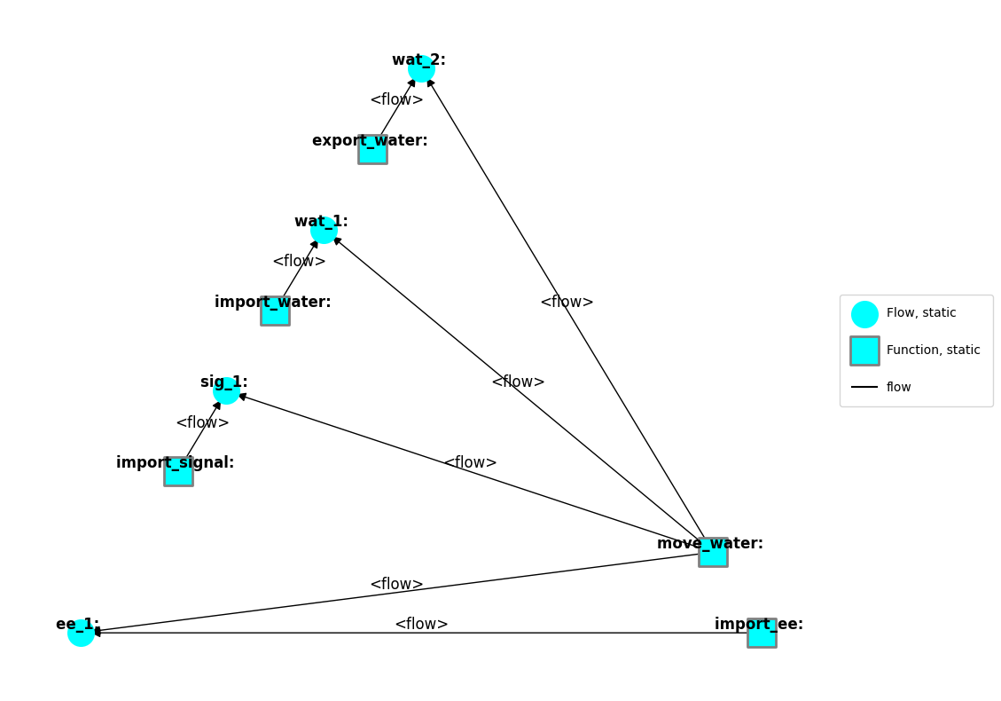
As shown, because all of the methods were defined as generic behaviors, they are each run in the static propagation step. No order is shown in the static step because the static propagation step iterates between model functions until the values have converged. Nevertheless, one can view the initial static order using:
mdl.staticsims
OrderedSet(['import_ee', 'import_water', 'import_signal', 'move_water', 'export_water'])
and the dynamic step order (if there was one):
mdl.dynamicsims
OrderedSet()
We can also instantiate this model with different parameters. In Pump model, these are defined in PumpParam
from ex_pump import PumpParam
p = PumpParam()
p
PumpParam(cost=('repair', 'water'), delay=10)
We can pass non-default parameters to the model (as well as other non-defaults, such as simulation parameters SimParam and random seeds) by passing them as dictionaries. In this case:
mdl2 = Pump(p={'cost':('repair', 'water', 'ee'), 'delay':20})
mdl2
pump Pump
- t=Time(time=-0.1, timers={})
- m=Mode(mode='nominal', faults=set(), sub_faults=False)
FLOWS:
- ee_1=Electricity(s=(current=1.0, voltage=1.0))
- sig_1=Signal(s=(power=1.0))
- wat_1=Water(s=(flowrate=1.0, pressure=1.0, area=1.0, level=1.0))
- wat_2=Water(s=(flowrate=1.0, pressure=1.0, area=1.0, level=1.0))
FXNS:
- import_ee=ImportEE(s=(effstate=1.0), m=(mode='nominal', faults=set(), sub_faults=False))
- import_water=ImportWater(m=(mode='nominal', faults=set(), sub_faults=False))
- import_signal=ImportSig(m=(mode='nominal', faults=set(), sub_faults=False))
- move_water=MoveWat(s=(eff=1.0), m=(mode='nominal', faults=set(), sub_faults=False))
- export_water=ExportWater(m=(mode='nominal', faults=set(), sub_faults=False))
Note that, for a model:
pis theParameterdefining non-mutable attributes (which do not change over a simulation)spis theSimParamdefining the simulation start, end, and end conditionsris theRanddefining random variables (e.g., for setting a seed)
2.), 3.), and 4.) Simulate and visualize the results!
Now, we will use the methods in propagate and the visualization modules in rd to simulate the model and visualize the results.
2a.) Simulate nominal
To simulate the model in the nominal scenario, use the propagate.nominal method, which returns:
endresults, which is a result (or a dict of multiple results) specified by the to_return option, e.g.:
‘classify’ (default), which provides the dict from
mdl.classify‘graph’ or
fmdtools.define.graph.Graphsubclass for the model.‘fxnname.varname’/’flowname.varname’: which gets the values of these variables at a the end
a list of the above arguments (to return a dict of multiple)
a dict of lists (for multiple over time), e.g.
{time:[varnames,... 'classify']}
and mdlhist, which is a history of model states specified by the track option. Some of these options include:
fxns’
‘flows’
‘all’
‘none’
‘valparams’ (model states specified in mdl.valparams),
or a dict of form:
{'functions':{'fxn1':'att1'}, 'flows':{'flow1':'att1'}}
result_nominal, mdlhist_nominal=propagate.nominal(Pump(track="all"), to_return="classify")
What do the results look like? Explore results structures using the to_returns and track arguments.
result_nominal
tend.classify.rate:                  1.0
tend.classify.cost:                  0.0
tend.classify.expected_cost:         0.0
Note that a Result can take arbitrary form based on what is produced in classify(). By default, we often return:
rate, which is the rate for the scenario calculated from the underlying fault probability model (defined in theModefor eachFunction),cost, which is some cost calculated based on the consequences of the scenarioexpected_cost, which is the expected value of the cost of the scenario (i.e.rate*cost).
mdlhist_nominal
i.finished:                    array(56)
i.on:                          array(56)
m.sub_faults:                  array(56)
time:                          array(56)
flows.ee_1.s.current:          array(56)
flows.ee_1.s.voltage:          array(56)
flows.sig_1.s.power:           array(56)
flows.wat_1.s.flowrate:        array(56)
flows.wat_1.s.pressure:        array(56)
flows.wat_1.s.area:            array(56)
flows.wat_1.s.level:           array(56)
flows.wat_2.s.flowrate:        array(56)
flows.wat_2.s.pressure:        array(56)
flows.wat_2.s.area:            array(56)
flows.wat_2.s.level:           array(56)
fxns.import_ee.s.effstate:     array(56)
fxns.import_ee.m.faults.inf_v: array(56)
fxns.import_ee.m.faults.no_v:  array(56)
fxns.import_ee.m.sub_faults:   array(56)
fxns.import_water.m.faults.less_wat: array(56)
fxns.import_water.m.faults.no_wat: array(56)
fxns.import_water.m.sub_faults: array(56)
fxns.import_signal.m.faults.no_sig: array(56)
fxns.import_signal.m.sub_faults: array(56)
fxns.move_water.i.over_pressure: array(56)
fxns.move_water.s.eff:         array(56)
fxns.move_water.m.faults.mech_break: array(56)
fxns.move_water.m.faults.short: array(56)
fxns.move_water.m.sub_faults:  array(56)
fxns.move_water.t.pressure_limit.time: array(56)
fxns.move_water.t.pressure_limit.mode: array(56)
fxns.export_water.m.faults.block: array(56)
fxns.export_water.m.sub_faults: array(56)
2b.) Visualize nominal model
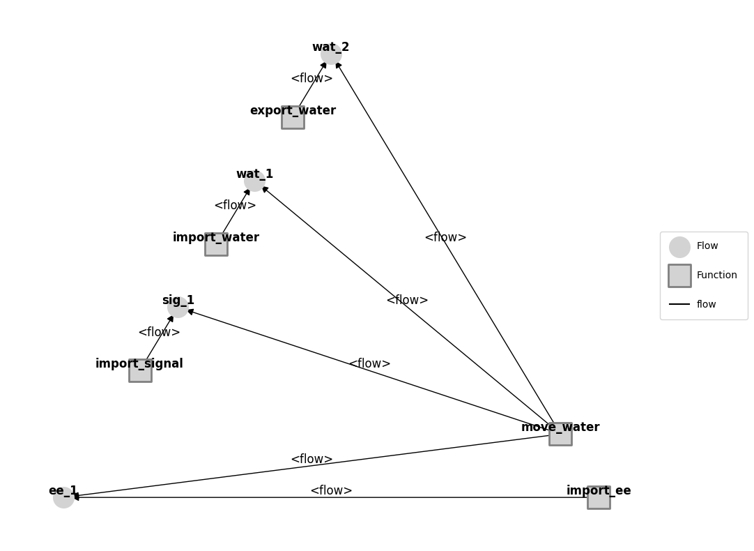
First, we can show the model graph using Graph.draw to see that it was set up correctly. We can do this both on the model graph itself (using ModelGraph) and the results of the nominal run (by passing graph as an argument in to_return) to verify both are fault-free.
Note that the underlying Graph classes are very flexible and enables a wide range of display options:
mg = mdl.as_modelgraph()
mg.draw()
(<Figure size 1200x1000 with 1 Axes>, <Axes: >)
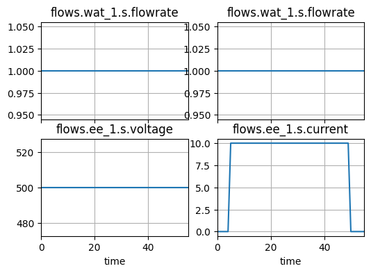
We can also view the flow values of the model using History.plot_line
It may be helpful to only view flows of interest.
fig = mdlhist_nominal.plot_line('flows.wat_1.s.flowrate', 'flows.wat_1.s.flowrate',
                                'flows.ee_1.s.voltage', 'flows.ee_1.s.current')
Note: for quick access to the syntax and options for these methods, type the ?method or help(method) in the terminal. For example ?History.plot_line
2b.) Simulate a fault mode
To simulate the model in a fault scenario, use the propagate.one_fault method. The set of possible faults is defined in the function definitions in ex_pump.py, and we can propagate a fault at any time in the operational interval (0-55 seconds).
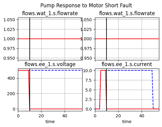
For example, below we simulate a short in the MoveWater function at time t=10:
results_fault, mdlhist_fault=propagate.one_fault(Pump(track="all"), 'move_water', 'short', time=10,
                                                 to_return=['classify', 'graph'])
We can also view the results for from this. In this case mdlhist gives a history of results for both the nominal and faulty runs.
results_fault
nominal.tend.classify.rate:          1.0
nominal.tend.classify.cost:          0.0
nominal.tend.classify.expected_cost: 0.0
nominal.tend.graph: <fmdtools.define.architecture.function.FunctionArchitectureGraph object at 0x00000226493A2350>
move_water_short_t10               1e-05
move_water_short_t10  29000.000000000007
move_water_short_t10  29000.000000000007
move_water_short_t10.tend.graph: <fmdtools.define.architecture.function.FunctionArchitectureGraph object at 0x00000226493A7590>
mdlhist_fault
nominal.i.finished:            array(56)
nominal.i.on:                  array(56)
nominal.m.sub_faults:          array(56)
nominal.time:                  array(56)
nominal.flows.ee_1.s.current:  array(56)
nominal.flows.ee_1.s.voltage:  array(56)
nominal.flows.sig_1.s.power:   array(56)
nominal.flows.wat_1.s.flowrate: array(56)
nominal.flows.wat_1.s.pressure: array(56)
nominal.flows.wat_1.s.area:    array(56)
nominal.flows.wat_1.s.level:   array(56)
nominal.flows.wat_2.s.flowrate: array(56)
nominal.flows.wat_2.s.pressure: array(56)
nominal.flows.wat_2.s.area:    array(56)
nominal.flows.wat_2.s.level:   array(56)
nominal.fxns.import_ee.s.effstate: array(56)
nominal.fxns.import_ee.m.faults.inf_v: array(56)
nominal.fxns.import_ee.m.faults.no_v: array(56)
nominal.fxns.import_ee.m.sub_faults: array(56)
nominal.fxns.import_           array(56)
nominal.fxns.import_           array(56)
nominal.fxns.import_water.m.sub_faults: array(56)
nominal.fxns.import_           array(56)
nominal.fxns.import_           array(56)
nominal.fxns.move_wa           array(56)
nominal.fxns.move_water.s.eff: array(56)
nominal.fxns.move_wa           array(56)
nominal.fxns.move_water.m.faults.short: array(56)
nominal.fxns.move_water.m.sub_faults: array(56)
nominal.fxns.move_wa           array(56)
nominal.fxns.move_wa           array(56)
nominal.fxns.export_           array(56)
nominal.fxns.export_water.m.sub_faults: array(56)
move_water_short_t10.i.finished: array(56)
move_water_short_t10.i.on:     array(56)
move_water_short_t10.m.sub_faults: array(56)
move_water_short_t10.time:     array(56)
move_water_short_t10           array(56)
move_water_short_t10           array(56)
move_water_short_t10           array(56)
move_water_short_t10           array(56)
move_water_short_t10           array(56)
move_water_short_t10           array(56)
move_water_short_t10           array(56)
move_water_short_t10           array(56)
move_water_short_t10           array(56)
move_water_short_t10           array(56)
move_water_short_t10           array(56)
move_water_short_t10           array(56)
move_water_short_t10           array(56)
move_water_short_t10           array(56)
move_water_short_t10           array(56)
move_water_short_t10           array(56)
move_water_short_t10           array(56)
move_water_short_t10           array(56)
move_water_short_t10           array(56)
move_water_short_t10           array(56)
move_water_short_t10           array(56)
move_water_short_t10           array(56)
move_water_short_t10           array(56)
move_water_short_t10           array(56)
move_water_short_t10           array(56)
move_water_short_t10           array(56)
move_water_short_t10           array(56)
move_water_short_t10           array(56)
move_water_short_t10           array(56)
3b.) Visualize fault model states
History.plot_line also works for a mdlhists given from propagate.one_fault. We can view these results below. As shown, the function will give the nominal result in a blue dotted line and the faulty result in a red line.
fig, axs = mdlhist_fault.plot_line('flows.wat_1.s.flowrate', 'flows.wat_1.s.flowrate',
                                   'flows.ee_1.s.voltage', 'flows.ee_1.s.current',
                                   title='Pump Response to Motor Short Fault',
                                   time_slice=[10], legend_loc=False)
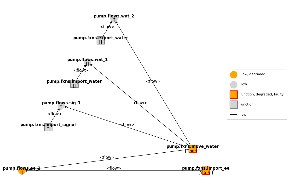
We can also view this result graph using Graph.draw. In this case, it shows the state of the model at the final time-step of the model run. Thus, while the EE_1 flow is shown in orange (because it is off-nominal), the Water flows are not, because they have the same state at the final time-step.
results_fault.faulty.tend.graph.draw()
(<Figure size 1200x1000 with 1 Axes>, <Axes: >)
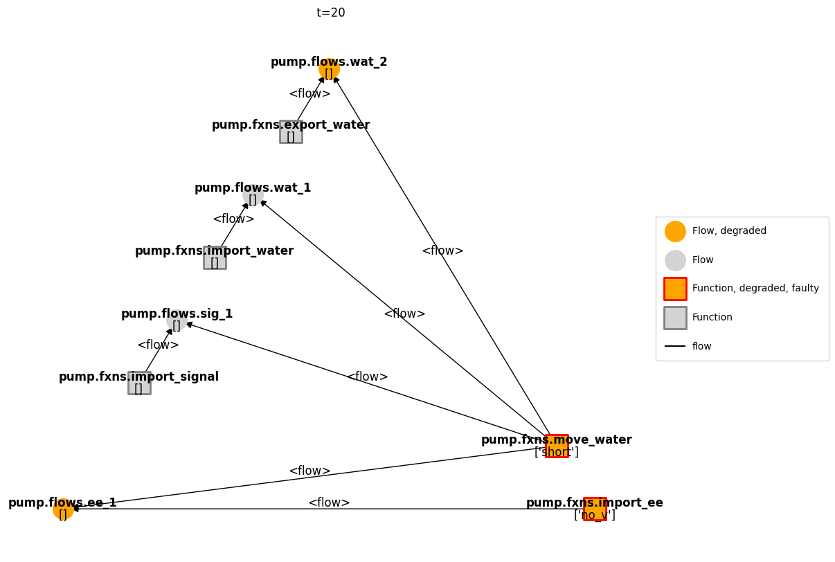
If we want to view the graph at another time-step, we can use Graph.draw_from, which will call History.get_degraded_hist to first process the model states into results which can be visualized and then map that onto a graph view at a given time.
fig, ax = mg.draw_from(20,mdlhist_fault)
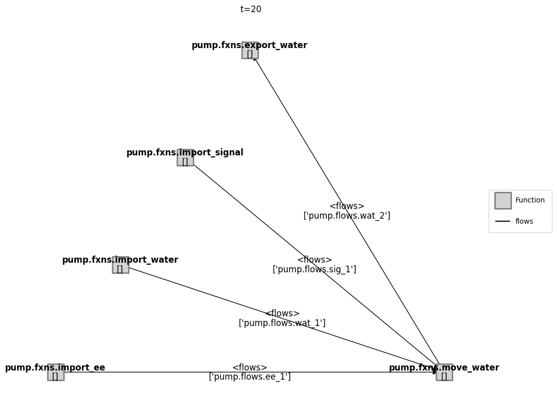
Note that multiple graph representations are available for the graph if desired…
from fmdtools.define.architecture.function import FunctionArchitectureFxnGraph
mg1 = FunctionArchitectureFxnGraph(mdl)
fig, ax = mg1.draw_from(20, mdlhist_fault, rem_ind=0)
4a.) Simulate set of fault modes
To simulate the set of fault modes, we first choose a FaultDomain and FaultSample. For simplicity, we can choose default parameters at first.
fd = FaultDomain(mdl)
fd.add_all()
fd
FaultDomain with faults:
 -('pump.fxns.import_ee', 'inf_v')
 -('pump.fxns.import_ee', 'no_v')
 -('pump.fxns.import_water', 'less_wat')
 -('pump.fxns.import_water', 'no_wat')
 -('pump.fxns.import_signal', 'no_sig')
 -('pump.fxns.move_water', 'mech_break')
 -('pump.fxns.move_water', 'short')
 -('pump.fxns.export_water', 'block')
fs = FaultSample(fd, phasemap = PhaseMap(mdl.sp.phases))
fs.add_fault_phases()
fs
FaultSample of scenarios:
 - pump_fxns_import_ee_inf_v_t2p0
 - pump_fxns_import_ee_no_v_t2p0
 - pump_fxns_import_water_less_wat_t2p0
 - pump_fxns_import_water_no_wat_t2p0
 - pump_fxns_import_signal_no_sig_t2p0
 - pump_fxns_move_water_mech_break_t2p0
 - pump_fxns_move_water_short_t2p0
 - pump_fxns_export_water_block_t2p0
 - pump_fxns_import_ee_inf_v_t27p0
 - pump_fxns_import_ee_no_v_t27p0
 - ... (24 total)
results_samp, mdlhists_samp = propagate.fault_sample(mdl, fs)
SCENARIOS COMPLETE: 100%|██████████| 24/24 [00:00<00:00, 40.59it/s]
It can be helpful to view what these results look like–a Result of faults injected at particular times with their correspnding Result dictionaries.
results_samp
nominal.tend.classify.rate:          1.0
nominal.tend.classify.cost:          0.0
nominal.tend.classify.expected_cost: 0.0
pump_fxns_import_ee_                 0.0
pump_fxns_import_ee_  25125.000000000007
pump_fxns_import_ee_                 0.0
pump_fxns_import_ee_                 0.0
pump_fxns_import_ee_  20125.000000000007
pump_fxns_import_ee_                 0.0
pump_fxns_import_wat               1e-05
pump_fxns_import_wat   5062.500000000004
pump_fxns_import_wat   5062.500000000004
pump_fxns_import_wat               1e-05
pump_fxns_import_wat  11125.000000000007
pump_fxns_import_wat  11125.000000000007
pump_fxns_import_sig             1.5e-06
pump_fxns_import_sig  20125.000000000007
pump_fxns_import_sig   3018.750000000001
pump_fxns_move_water6.000000000000001e-07
pump_fxns_move_water  15125.000000000007
pump_fxns_move_water   907.5000000000005
pump_fxns_move_water1.5000000000000002e-05
pump_fxns_move_water  30125.000000000007
pump_fxns_move_water  45187.500000000015
pump_fxns_export_wat1.5000000000000002e-05
pump_fxns_export_wat  20102.500000000007
pump_fxns_export_wat  30153.750000000015
pump_fxns_import_ee_2.0000000000000003e-06
pump_fxns_import_ee_             20175.0
pump_fxns_import_ee_   4035.000000000001
pump_fxns_import_ee_8.000000000000001e-06
pump_fxns_import_ee_  15174.999999999998
pump_fxns_import_ee_             12140.0
pump_fxns_import_wat               1e-05
pump_fxns_import_wat   2587.499999999999
pump_fxns_import_wat   2587.499999999999
pump_fxns_import_wat               1e-05
pump_fxns_import_wat   6174.999999999998
pump_fxns_import_wat   6174.999999999998
pump_fxns_import_sig               1e-06
pump_fxns_import_sig  15174.999999999998
pump_fxns_import_sig  1517.4999999999998
pump_fxns_move_water             7.2e-06
pump_fxns_move_water  10174.999999999998
pump_fxns_move_water   7325.999999999998
pump_fxns_move_water               1e-05
pump_fxns_move_water             25175.0
pump_fxns_move_water             25175.0
pump_fxns_export_wat               1e-05
pump_fxns_export_wat             15152.5
pump_fxns_export_wat             15152.5
pump_fxns_import_ee_                 0.0
pump_fxns_import_ee_              5000.0
pump_fxns_import_ee_                 0.0
pump_fxns_import_ee_                 0.0
pump_fxns_import_ee_             10000.0
pump_fxns_import_ee_                 0.0
pump_fxns_import_wat               1e-05
pump_fxns_import_wat                 0.0
pump_fxns_import_wat                 0.0
pump_fxns_import_wat               1e-05
pump_fxns_import_wat              1000.0
pump_fxns_import_wat              1000.0
pump_fxns_import_sig               1e-06
pump_fxns_import_sig             10000.0
pump_fxns_import_sig   999.9999999999999
pump_fxns_move_water6.000000000000001e-07
pump_fxns_move_water              5000.0
pump_fxns_move_water               300.0
pump_fxns_move_water               1e-05
pump_fxns_move_water             10000.0
pump_fxns_move_water             10000.0
pump_fxns_export_wat               1e-05
pump_fxns_export_wat              5000.0
pump_fxns_export_wat              5000.0
We can look at/use a more structured version using:
ec_nest = results_samp.nest()
ec_nest
nominal:
--tend:
----classify:
------rate:                          1.0
------cost:                          0.0
------expected_cost:                 0.0
pump_fxns_import_ee_inf_v_t2p0:
--tend:
----classify:
------rate:                          0.0
------cost:           25125.000000000007
------expected_cost:                 0.0
pump_fxns_import_ee_no_v_t2p0:
--tend:
----classify:
------rate:                          0.0
------cost:           20125.000000000007
------expected_cost:                 0.0
pump_fxns_import_water_less_wat_t2p0:
--tend:
----classify:
------rate:                        1e-05
------cost:            5062.500000000004
------expected_cost:   5062.500000000004
pump_fxns_import_water_no_wat_t2p0:
--tend:
----classify:
------rate:                        1e-05
------cost:           11125.000000000007
------expected_cost:  11125.000000000007
pump_fxns_import_signal_no_sig_t2p0:
--tend:
----classify:
------rate:                      1.5e-06
------cost:           20125.000000000007
------expected_cost:   3018.750000000001
pump_fxns_move_water_mech_break_t2p0:
--tend:
----classify:
------rate:        6.000000000000001e-07
------cost:           15125.000000000007
------expected_cost:   907.5000000000005
pump_fxns_move_water_short_t2p0:
--tend:
----classify:
------rate:       1.5000000000000002e-05
------cost:           30125.000000000007
------expected_cost:  45187.500000000015
pump_fxns_export_water_block_t2p0:
--tend:
----classify:
------rate:       1.5000000000000002e-05
------cost:           20102.500000000007
------expected_cost:  30153.750000000015
pump_fxns_import_ee_inf_v_t27p0:
--tend:
----classify:
------rate:       2.0000000000000003e-06
------cost:                      20175.0
------expected_cost:   4035.000000000001
pump_fxns_import_ee_no_v_t27p0:
--tend:
----classify:
------rate:        8.000000000000001e-06
------cost:           15174.999999999998
------expected_cost:             12140.0
pump_fxns_import_water_less_wat_t27p0:
--tend:
----classify:
------rate:                        1e-05
------cost:            2587.499999999999
------expected_cost:   2587.499999999999
pump_fxns_import_water_no_wat_t27p0:
--tend:
----classify:
------rate:                        1e-05
------cost:            6174.999999999998
------expected_cost:   6174.999999999998
pump_fxns_import_signal_no_sig_t27p0:
--tend:
----classify:
------rate:                        1e-06
------cost:           15174.999999999998
------expected_cost:  1517.4999999999998
pump_fxns_move_water_mech_break_t27p0:
--tend:
----classify:
------rate:                      7.2e-06
------cost:           10174.999999999998
------expected_cost:   7325.999999999998
pump_fxns_move_water_short_t27p0:
--tend:
----classify:
------rate:                        1e-05
------cost:                      25175.0
------expected_cost:             25175.0
pump_fxns_export_water_block_t27p0:
--tend:
----classify:
------rate:                        1e-05
------cost:                      15152.5
------expected_cost:             15152.5
pump_fxns_import_ee_inf_v_t52p0:
--tend:
----classify:
------rate:                          0.0
------cost:                       5000.0
------expected_cost:                 0.0
pump_fxns_import_ee_no_v_t52p0:
--tend:
----classify:
------rate:                          0.0
------cost:                      10000.0
------expected_cost:                 0.0
pump_fxns_import_water_less_wat_t52p0:
--tend:
----classify:
------rate:                        1e-05
------cost:                          0.0
------expected_cost:                 0.0
pump_fxns_import_water_no_wat_t52p0:
--tend:
----classify:
------rate:                        1e-05
------cost:                       1000.0
------expected_cost:              1000.0
pump_fxns_import_signal_no_sig_t52p0:
--tend:
----classify:
------rate:                        1e-06
------cost:                      10000.0
------expected_cost:   999.9999999999999
pump_fxns_move_water_mech_break_t52p0:
--tend:
----classify:
------rate:        6.000000000000001e-07
------cost:                       5000.0
------expected_cost:               300.0
pump_fxns_move_water_short_t52p0:
--tend:
----classify:
------rate:                        1e-05
------cost:                      10000.0
------expected_cost:             10000.0
pump_fxns_export_water_block_t52p0:
--tend:
----classify:
------rate:                        1e-05
------cost:                       5000.0
------expected_cost:              5000.0
We often want to adjust the FaultDomain and SampleApproach to answer specific questions about the model (e.g. focussing on single faults, different numbers of sample points, etc). Both have different methods with options which can be changed to enable this, e.g.:
fd2 = FaultDomain(mdl)
fd2.add_fault('move_water', 'short')
fd2
FaultDomain with faults:
 -('move_water', 'short')
fs2 = FaultSample(fd2, phasemap = PhaseMap(mdl.sp.phases))
fs2.add_fault_phases(args=(4,))
fs2
FaultSample of scenarios:
 - move_water_short_t0p0
 - move_water_short_t1p0
 - move_water_short_t2p0
 - move_water_short_t3p0
 - move_water_short_t4p0
 - move_water_short_t14p0
 - move_water_short_t23p0
 - move_water_short_t31p0
 - move_water_short_t40p0
 - move_water_short_t51p0
 - ... (13 total)
There are a number of different ways to sample the scenarios in the approach:
fs2.get_times()
[0.0, 1.0, 2.0, 3.0, 4.0, 40.0, 14.0, 51.0, 52.0, 53.0, 54.0, 23.0, 31.0]
4b.) Visualize set of fault modes
Using this fault approach, we can now make an FMEA-like analyses of the different fault modes. The an.tabulate.FMEA class organizes results such that you can create a table (or plot) for each fault.
summary_fmea = an.tabulate.FMEA(results_samp, fs)
summary_fmea.as_table()
| average_scenario_rate | sum_cost | expected_cost | ||
|---|---|---|---|---|
| pump.fxns.move_water | short | 1.166667e-05 | 65300.0 | 0.803625 |
| pump.fxns.export_water | block | 1.166667e-05 | 40255.0 | 0.503063 |
| pump.fxns.import_water | no_wat | 1.000000e-05 | 18300.0 | 0.183000 |
| pump.fxns.import_ee | no_v | 2.666667e-06 | 45300.0 | 0.121400 |
| pump.fxns.move_water | mech_break | 2.800000e-06 | 30300.0 | 0.085335 |
| pump.fxns.import_water | less_wat | 1.000000e-05 | 7650.0 | 0.076500 |
| pump.fxns.import_signal | no_sig | 1.166667e-06 | 45300.0 | 0.055363 |
| pump.fxns.import_ee | inf_v | 6.666667e-07 | 50300.0 | 0.040350 |
We can also use an.tabulate.result_summary_fmea with the processed results histories to get a better picture of which flows and functions degrade in each scenario.
an.tabulate.result_summary_fmea(results_samp, mdlhists_samp, *mdl.fxns, *mdl.flows)
| degraded | faulty | rate | cost | expected_cost | |
|---|---|---|---|---|---|
| nominal | [] | [] | 1.0 | 0.0 | 0.0 |
| pump_fxns_import_ee_inf_v_t2p0 | ['ee_1', 'wat_2'] | [] | 0.0 | 25125.0 | 0.0 |
| pump_fxns_import_ee_no_v_t2p0 | ['ee_1', 'wat_2'] | [] | 0.0 | 20125.0 | 0.0 |
| pump_fxns_import_water_less_wat_t2p0 | ['ee_1', 'wat_2'] | [] | 0.00001 | 5062.5 | 5062.5 |
| pump_fxns_import_water_no_wat_t2p0 | ['ee_1', 'wat_2'] | [] | 0.00001 | 11125.0 | 11125.0 |
| pump_fxns_import_signal_no_sig_t2p0 | ['ee_1', 'wat_2'] | [] | 0.000002 | 20125.0 | 3018.75 |
| pump_fxns_move_water_mech_break_t2p0 | ['ee_1', 'wat_2'] | [] | 0.000001 | 15125.0 | 907.5 |
| pump_fxns_move_water_short_t2p0 | ['ee_1', 'wat_2'] | [] | 0.000015 | 30125.0 | 45187.5 |
| pump_fxns_export_water_block_t2p0 | ['ee_1', 'wat_2'] | [] | 0.000015 | 20102.5 | 30153.75 |
| pump_fxns_import_ee_inf_v_t27p0 | ['ee_1', 'wat_2'] | [] | 0.000002 | 20175.0 | 4035.0 |
| pump_fxns_import_ee_no_v_t27p0 | ['ee_1', 'wat_2'] | [] | 0.000008 | 15175.0 | 12140.0 |
| pump_fxns_import_water_less_wat_t27p0 | ['ee_1', 'wat_2'] | [] | 0.00001 | 2587.5 | 2587.5 |
| pump_fxns_import_water_no_wat_t27p0 | ['ee_1', 'wat_2'] | [] | 0.00001 | 6175.0 | 6175.0 |
| pump_fxns_import_signal_no_sig_t27p0 | ['ee_1', 'wat_2'] | [] | 0.000001 | 15175.0 | 1517.5 |
| pump_fxns_move_water_mech_break_t27p0 | ['ee_1', 'wat_2'] | [] | 0.000007 | 10175.0 | 7326.0 |
| pump_fxns_move_water_short_t27p0 | ['ee_1', 'wat_2'] | [] | 0.00001 | 25175.0 | 25175.0 |
| pump_fxns_export_water_block_t27p0 | ['ee_1', 'wat_2'] | [] | 0.00001 | 15152.5 | 15152.5 |
| pump_fxns_import_ee_inf_v_t52p0 | [] | [] | 0.0 | 5000.0 | 0.0 |
| pump_fxns_import_ee_no_v_t52p0 | [] | [] | 0.0 | 10000.0 | 0.0 |
| pump_fxns_import_water_less_wat_t52p0 | [] | [] | 0.00001 | 0.0 | 0.0 |
| pump_fxns_import_water_no_wat_t52p0 | [] | [] | 0.00001 | 1000.0 | 1000.0 |
| pump_fxns_import_signal_no_sig_t52p0 | [] | [] | 0.000001 | 10000.0 | 1000.0 |
| pump_fxns_move_water_mech_break_t52p0 | [] | [] | 0.000001 | 5000.0 | 300.0 |
| pump_fxns_move_water_short_t52p0 | [] | [] | 0.00001 | 10000.0 | 10000.0 |
| pump_fxns_export_water_block_t52p0 | [] | [] | 0.00001 | 5000.0 | 5000.0 |
Note that this is contingent on what we tracked in the history! In the above model, we used the default, which is only a few variables defined in the model.
If we tracked all, on the other hand, we would get the result below:
results_samp, mdlhists_samp = propagate.fault_sample(mdl, fs, track="all")
an.tabulate.result_summary_fmea(results_samp, mdlhists_samp, *mdl.fxns, *mdl.flows)
SCENARIOS COMPLETE: 100%|██████████| 24/24 [00:00<00:00, 38.66it/s]
| degraded | faulty | rate | cost | expected_cost | |
|---|---|---|---|---|---|
| nominal | [] | [] | 1.0 | 0.0 | 0.0 |
| pump_fxns_import_ee_inf_v_t2p0 | ['ee_1', 'wat_2'] | [] | 0.0 | 25125.0 | 0.0 |
| pump_fxns_import_ee_no_v_t2p0 | ['ee_1', 'wat_2'] | [] | 0.0 | 20125.0 | 0.0 |
| pump_fxns_import_water_less_wat_t2p0 | ['ee_1', 'wat_2'] | [] | 0.00001 | 5062.5 | 5062.5 |
| pump_fxns_import_water_no_wat_t2p0 | ['ee_1', 'wat_2'] | [] | 0.00001 | 11125.0 | 11125.0 |
| pump_fxns_import_signal_no_sig_t2p0 | ['ee_1', 'wat_2'] | [] | 0.000002 | 20125.0 | 3018.75 |
| pump_fxns_move_water_mech_break_t2p0 | ['ee_1', 'wat_2'] | [] | 0.000001 | 15125.0 | 907.5 |
| pump_fxns_move_water_short_t2p0 | ['ee_1', 'wat_2'] | [] | 0.000015 | 30125.0 | 45187.5 |
| pump_fxns_export_water_block_t2p0 | ['ee_1', 'wat_2'] | [] | 0.000015 | 20102.5 | 30153.75 |
| pump_fxns_import_ee_inf_v_t27p0 | ['ee_1', 'wat_2'] | [] | 0.000002 | 20175.0 | 4035.0 |
| pump_fxns_import_ee_no_v_t27p0 | ['ee_1', 'wat_2'] | [] | 0.000008 | 15175.0 | 12140.0 |
| pump_fxns_import_water_less_wat_t27p0 | ['ee_1', 'wat_2'] | [] | 0.00001 | 2587.5 | 2587.5 |
| pump_fxns_import_water_no_wat_t27p0 | ['ee_1', 'wat_2'] | [] | 0.00001 | 6175.0 | 6175.0 |
| pump_fxns_import_signal_no_sig_t27p0 | ['ee_1', 'wat_2'] | [] | 0.000001 | 15175.0 | 1517.5 |
| pump_fxns_move_water_mech_break_t27p0 | ['ee_1', 'wat_2'] | [] | 0.000007 | 10175.0 | 7326.0 |
| pump_fxns_move_water_short_t27p0 | ['ee_1', 'wat_2'] | [] | 0.00001 | 25175.0 | 25175.0 |
| pump_fxns_export_water_block_t27p0 | ['ee_1', 'wat_2'] | [] | 0.00001 | 15152.5 | 15152.5 |
| pump_fxns_import_ee_inf_v_t52p0 | [] | [] | 0.0 | 5000.0 | 0.0 |
| pump_fxns_import_ee_no_v_t52p0 | [] | [] | 0.0 | 10000.0 | 0.0 |
| pump_fxns_import_water_less_wat_t52p0 | [] | [] | 0.00001 | 0.0 | 0.0 |
| pump_fxns_import_water_no_wat_t52p0 | [] | [] | 0.00001 | 1000.0 | 1000.0 |
| pump_fxns_import_signal_no_sig_t52p0 | [] | [] | 0.000001 | 10000.0 | 1000.0 |
| pump_fxns_move_water_mech_break_t52p0 | [] | [] | 0.000001 | 5000.0 | 300.0 |
| pump_fxns_move_water_short_t52p0 | [] | [] | 0.00001 | 10000.0 | 10000.0 |
| pump_fxns_export_water_block_t52p0 | [] | [] | 0.00001 | 5000.0 | 5000.0 |
5.) Saving Work
In computationally expensive simulations, running a lot of computational simulations can take a considerable amount of time. As a result, it becomes impractical to run a new simulation every time one wishes to analyse its data. Results from fmdtools simulations (Result or History) can be saved as npz, csv, or json files in this instance using either:
Result.save/History.saveorpassing a save_args dictionary to the respective propagate functions (e.g.,
{'classify':{'filename':'file.pkl','overwrite':True})
and then loaded using:
Result.load/History.load
For example, for this variable:
results_samp
nominal.tend.classify.rate:          1.0
nominal.tend.classify.cost:          0.0
nominal.tend.classify.expected_cost: 0.0
pump_fxns_import_ee_                 0.0
pump_fxns_import_ee_  25125.000000000007
pump_fxns_import_ee_                 0.0
pump_fxns_import_ee_                 0.0
pump_fxns_import_ee_  20125.000000000007
pump_fxns_import_ee_                 0.0
pump_fxns_import_wat               1e-05
pump_fxns_import_wat   5062.500000000004
pump_fxns_import_wat   5062.500000000004
pump_fxns_import_wat               1e-05
pump_fxns_import_wat  11125.000000000007
pump_fxns_import_wat  11125.000000000007
pump_fxns_import_sig             1.5e-06
pump_fxns_import_sig  20125.000000000007
pump_fxns_import_sig   3018.750000000001
pump_fxns_move_water6.000000000000001e-07
pump_fxns_move_water  15125.000000000007
pump_fxns_move_water   907.5000000000005
pump_fxns_move_water1.5000000000000002e-05
pump_fxns_move_water  30125.000000000007
pump_fxns_move_water  45187.500000000015
pump_fxns_export_wat1.5000000000000002e-05
pump_fxns_export_wat  20102.500000000007
pump_fxns_export_wat  30153.750000000015
pump_fxns_import_ee_2.0000000000000003e-06
pump_fxns_import_ee_             20175.0
pump_fxns_import_ee_   4035.000000000001
pump_fxns_import_ee_8.000000000000001e-06
pump_fxns_import_ee_  15174.999999999998
pump_fxns_import_ee_             12140.0
pump_fxns_import_wat               1e-05
pump_fxns_import_wat   2587.499999999999
pump_fxns_import_wat   2587.499999999999
pump_fxns_import_wat               1e-05
pump_fxns_import_wat   6174.999999999998
pump_fxns_import_wat   6174.999999999998
pump_fxns_import_sig               1e-06
pump_fxns_import_sig  15174.999999999998
pump_fxns_import_sig  1517.4999999999998
pump_fxns_move_water             7.2e-06
pump_fxns_move_water  10174.999999999998
pump_fxns_move_water   7325.999999999998
pump_fxns_move_water               1e-05
pump_fxns_move_water             25175.0
pump_fxns_move_water             25175.0
pump_fxns_export_wat               1e-05
pump_fxns_export_wat             15152.5
pump_fxns_export_wat             15152.5
pump_fxns_import_ee_                 0.0
pump_fxns_import_ee_              5000.0
pump_fxns_import_ee_                 0.0
pump_fxns_import_ee_                 0.0
pump_fxns_import_ee_             10000.0
pump_fxns_import_ee_                 0.0
pump_fxns_import_wat               1e-05
pump_fxns_import_wat                 0.0
pump_fxns_import_wat                 0.0
pump_fxns_import_wat               1e-05
pump_fxns_import_wat              1000.0
pump_fxns_import_wat              1000.0
pump_fxns_import_sig               1e-06
pump_fxns_import_sig             10000.0
pump_fxns_import_sig   999.9999999999999
pump_fxns_move_water6.000000000000001e-07
pump_fxns_move_water              5000.0
pump_fxns_move_water               300.0
pump_fxns_move_water               1e-05
pump_fxns_move_water             10000.0
pump_fxns_move_water             10000.0
pump_fxns_export_wat               1e-05
pump_fxns_export_wat              5000.0
pump_fxns_export_wat              5000.0
results_samp.save('tutorial_results.csv', overwrite=True)
File already exists: tutorial_endclasses.csv, writing anyway...
results_saved = an.result.Result.load('tutorial_endclasses.csv')
results_saved
nominal.tend.classify.rate:          1.0
nominal.tend.classify.cost:          0.0
nominal.tend.classify.expected_cost: 0.0
pump_fxns_import_ee_                 0.0
pump_fxns_import_ee_  25125.000000000007
pump_fxns_import_ee_                 0.0
pump_fxns_import_ee_                 0.0
pump_fxns_import_ee_  20125.000000000007
pump_fxns_import_ee_                 0.0
pump_fxns_import_wat               1e-05
pump_fxns_import_wat   5062.500000000004
pump_fxns_import_wat   5062.500000000004
pump_fxns_import_wat               1e-05
pump_fxns_import_wat  11125.000000000007
pump_fxns_import_wat  11125.000000000007
pump_fxns_import_sig             1.5e-06
pump_fxns_import_sig  20125.000000000007
pump_fxns_import_sig   3018.750000000001
pump_fxns_move_water6.000000000000001e-07
pump_fxns_move_water  15125.000000000007
pump_fxns_move_water   907.5000000000005
pump_fxns_move_water1.5000000000000002e-05
pump_fxns_move_water  30125.000000000007
pump_fxns_move_water  45187.500000000015
pump_fxns_export_wat1.5000000000000002e-05
pump_fxns_export_wat  20102.500000000007
pump_fxns_export_wat   30153.75000000001
pump_fxns_import_ee_2.0000000000000003e-06
pump_fxns_import_ee_             20175.0
pump_fxns_import_ee_   4035.000000000001
pump_fxns_import_ee_8.000000000000001e-06
pump_fxns_import_ee_  15174.999999999998
pump_fxns_import_ee_             12140.0
pump_fxns_import_wat               1e-05
pump_fxns_import_wat   2587.499999999999
pump_fxns_import_wat   2587.499999999999
pump_fxns_import_wat               1e-05
pump_fxns_import_wat   6174.999999999998
pump_fxns_import_wat   6174.999999999998
pump_fxns_import_sig               1e-06
pump_fxns_import_sig  15174.999999999998
pump_fxns_import_sig  1517.4999999999998
pump_fxns_move_water             7.2e-06
pump_fxns_move_water  10174.999999999998
pump_fxns_move_water   7325.999999999998
pump_fxns_move_water               1e-05
pump_fxns_move_water             25175.0
pump_fxns_move_water             25175.0
pump_fxns_export_wat               1e-05
pump_fxns_export_wat             15152.5
pump_fxns_export_wat             15152.5
pump_fxns_import_ee_                 0.0
pump_fxns_import_ee_              5000.0
pump_fxns_import_ee_                 0.0
pump_fxns_import_ee_                 0.0
pump_fxns_import_ee_             10000.0
pump_fxns_import_ee_                 0.0
pump_fxns_import_wat               1e-05
pump_fxns_import_wat                 0.0
pump_fxns_import_wat                 0.0
pump_fxns_import_wat               1e-05
pump_fxns_import_wat              1000.0
pump_fxns_import_wat              1000.0
pump_fxns_import_sig               1e-06
pump_fxns_import_sig             10000.0
pump_fxns_import_sig              1000.0
pump_fxns_move_water6.000000000000001e-07
pump_fxns_move_water              5000.0
pump_fxns_move_water               300.0
pump_fxns_move_water               1e-05
pump_fxns_move_water             10000.0
pump_fxns_move_water             10000.0
pump_fxns_export_wat               1e-05
pump_fxns_export_wat              5000.0
pump_fxns_export_wat              5000.0