Defining Fault Sampling Approaches in fmdtools
Fault Sampling is used to evaluate the overall resilience of a system to a set of faults and the corresponding risks associated with these faults. There is no single best way to define the set of scenarios to evaluate resilience with, because a given resilience analysis may need more or less detail, support more or less computational time, or be interested in specific scenario types of interest.
Thus, there are a number of use-cases supported by fmdtools for different sampling models. This document will demonstrate and showcase a few of them.
Copyright © 2024, United States Government, as represented by the Administrator of the National Aeronautics and Space Administration. All rights reserved.

The “"Fault Model Design tools - fmdtools version 2"” software is licensed under the Apache License, Version 2.0 (the "License"); you may not use this file except in compliance with the License. You may obtain a copy of the License at http://www.apache.org/licenses/LICENSE-2.0.

Unless required by applicable law or agreed to in writing, software distributed under the License is distributed on an "AS IS" BASIS, WITHOUT WARRANTIES OR CONDITIONS OF ANY KIND, either express or implied. See the License for the specific language governing permissions and limitations under the License.
from fmdtools.sim.sample import SampleApproach, FaultSample, FaultDomain
from fmdtools.analyze.tabulate import FMEA, Comparison
import fmdtools.sim.propagate as prop
import numpy as np
Basics
Fault sampling involves:
Defining faults and fault models for each function/component/flows of the model is done using the ‘Mode’ Class
Defining a fault sampling approach, using the:
SampleApproachclass, orFaultDomainandFaultSamplecalsses directly
Propagating faults through the model (using the
propagate.faultsamplemethod) Before proceeding, it can be helpful to look through their respective documentation.
Model Setup
Consider the rover model in rover_model
import inspect
from rover_model import Power, PowerMode
This rover has a Power function:
print(inspect.getsource(Power))
class Power(Function):
    """Rover power supply."""

    __slots__ = ("ee_15", "ee_5", "ee_12", "switch")
    container_s = PowerState
    container_m = PowerMode
    flow_ee_15 = EE
    flow_ee_5 = EE
    flow_ee_12 = EE
    flow_switch = Switch

    def static_behavior(self, time):
        """Determine power use based on mode."""
        if self.m.in_mode("off"):
            self.off_power()
        elif self.m.in_mode("supply", "depleted"):
            self.supply_power()
        elif self.m.in_mode("short"):
            self.short_power()
        elif self.m.in_mode("no_charge"):
            self.no_charge_power()

        if self.m.in_mode("charge"):
            self.charge_power_usage()
        else:
            self.power_usage()
            if self.m.in_mode("short"):
                self.short_power_usage()

    def dynamic_behavior(self, time):
        """Charge increment over time."""
        self.s.inc(charge=-self.s.power / 100)
        self.s.limit(charge=(0, 100))

    def short_power(self):
        """Short in power supply means now power provided."""
        if self.s.charge > 0.1:
            self.ee_5.s.v = 5
            self.ee_12.s.v = 12
            self.ee_15.s.v = 15
        else:
            self.no_charge_power()

    def no_charge_power(self):
        """Battery is out of charge."""
        self.ee_5.s.v = 0
        self.ee_12.s.v = 0
        self.ee_15.s.v = 0

    def off_power(self):
        """Power supply is shut off."""
        self.ee_5.s.put(v=0, a=0)
        self.ee_12.s.put(v=0, a=0)
        self.ee_15.s.put(v=0, a=0)
        if self.switch.s.power:
            self.m.set_mode("supply")

    def supply_power(self):
        """Power supply is in supply mode."""
        if self.s.charge > 0:
            self.ee_5.s.v = 5
            self.ee_12.s.v = 12
            self.ee_15.s.v = 15
        else:
            self.m.to_fault("no_charge")
        if not self.switch.s.power:
            if not self.m.any_faults():
                self.m.set_mode("off")

    def power_usage(self):
        """Calculate the power usage in general."""
        self.s.power = (1.0 + self.ee_12.s.mul("v", "a") +
                        self.ee_5.s.mul("v", "a") + self.ee_15.s.mul("v", "a"))

    def charge_power_usage(self):
        """Calculate the power usage when the battery charges."""
        self.s.power = -1
        if self.s.charge == 100:
            self.m.set_mode("off")

    def short_power_usage(self):
        """Calculate power usage when there is a short (calculated as 10x)."""
        self.s.power = self.s.power * 10
Which contains the mode PowerMode:
print(inspect.getsource(PowerMode))
class PowerMode(Mode):
    """
    Possible modes for Power function.

    Modes
    -------
    no_charge : Fault
        Battery is out of charge.
    short: Fault
        There is a short.
    depletion: Fault
        The battery is depleted to a given percent
    supply: Mode
        supply power
    charge: Mode
        charge battery
    standby: Mode
        power supply is in stand by
    off: Mode
        power supply is off
    """

    fault_no_charge = (1e-5, 100, (("off", 1.0),))
    fault_short = (1e-5, 100, (("supply", 1.0),))
    fault_depleted: dict = {'disturbances': {'s.charge': 20.0}}
    opermodes = ("supply", "charge", "off")
    mode: str = "off"
    exclusive = True
The fault_faultname class variables specify three possible fault modes to inject, including “no_charge”, and “short”. More information has been added in the tuples defining each Fault, including:
rate
repair cost
phase dictionary The phase dictionary is important because it specifies that this mode is to occur in a given phase. In this case,
no_chargeis supposed to only occur during thestandbyphase whileshortis only supposed to occur during thesupplyphase. In thisMode, these phases correspond to the operational modes (opermodes), but they may correspond to other operational modes also.
All of these fields are optional, but they do help us develop a more informed statistical sample of the fault modes.
Setting up a FaultSample
Sampling using FaultSample first requires creating a FaultDomain to sample from. These faultdomains can be created from both models and individual functions:
fd_power = FaultDomain(Power())
fd_power.add_all()
fd_power
FaultDomain with faults:
 -('power', 'depleted')
 -('power', 'no_charge')
 -('power', 'short')
from rover_model import Rover
fd_rvr = FaultDomain(Rover())
fd_rvr.add_all()
fd_rvr
FaultDomain with faults:
 -('rover.fxns.power', 'depleted')
 -('rover.fxns.power', 'no_charge')
 -('rover.fxns.power', 'short')
 -('rover.fxns.perception', 'bad_feed')
 -('rover.fxns.plan_path', 'crash')
 -('rover.fxns.plan_path', 'no_con')
 -('rover.fxns.drive', 'custom')
 -('rover.fxns.drive', 'elec_open')
 -('rover.fxns.drive', 'stuck')
 -('rover.fxns.drive', 'stuck_left')
 -...more
Note that there are several methods in FaultDomain which let us specify the list of faults we want to sample from, e.g.:
fd_short = FaultDomain(Rover())
fd_short.add_all_modes("short")
fd_short
FaultDomain with faults:
 -('rover.fxns.power', 'short')
or:
fd_pwr = FaultDomain(Rover())
fd_pwr.add_all_fxn_modes("power")
fd_pwr
FaultDomain with faults:
 -('rover.fxns.power', 'depleted')
 -('rover.fxns.power', 'no_charge')
 -('rover.fxns.power', 'short')
We can then sample this domain using a FaultSample:
fs_pwr = FaultSample(fd_pwr, def_mdl_phasemap=False)
Note that FaultSamples have two main variables: faultdomain and phasemap. A PhaseMap is essentially a dictionary of phases to sample from.
In the above case, we don’t want to use phase information to form the sample, so we don’t provide any and we set def_mdl_phasemap=False, since this would get phase information from the model.
To add scenarios to the FaultSample, we can then use one of the add methods:
fs_pwr.add_fault_times([2,5,10])
fs_pwr
FaultSample of scenarios:
 - rover_fxns_power_depleted_t2
 - rover_fxns_power_depleted_t5
 - rover_fxns_power_depleted_t10
 - rover_fxns_power_no_charge_t2
 - rover_fxns_power_no_charge_t5
 - rover_fxns_power_no_charge_t10
 - rover_fxns_power_short_t2
 - rover_fxns_power_short_t5
 - rover_fxns_power_short_t10
As shown, this adds the list of faults in the faultdomain over the given times.
Note the underlying rate information in these scenarios is all the same:
fs_pwr.scenarios()
[SingleFaultScenario(sequence={2.0: Injection(faults={'rover.fxns.power': ['depleted']}, disturbances={})}, times=(2,), function='rover.fxns.power', fault='depleted', rate=1.0, name='rover_fxns_power_depleted_t2', time=2, phase=''),
 SingleFaultScenario(sequence={5.0: Injection(faults={'rover.fxns.power': ['depleted']}, disturbances={})}, times=(5,), function='rover.fxns.power', fault='depleted', rate=1.0, name='rover_fxns_power_depleted_t5', time=5, phase=''),
 SingleFaultScenario(sequence={10.0: Injection(faults={'rover.fxns.power': ['depleted']}, disturbances={})}, times=(10,), function='rover.fxns.power', fault='depleted', rate=1.0, name='rover_fxns_power_depleted_t10', time=10, phase=''),
 SingleFaultScenario(sequence={2.0: Injection(faults={'rover.fxns.power': ['no_charge']}, disturbances={})}, times=(2,), function='rover.fxns.power', fault='no_charge', rate=1e-05, name='rover_fxns_power_no_charge_t2', time=2, phase=''),
 SingleFaultScenario(sequence={5.0: Injection(faults={'rover.fxns.power': ['no_charge']}, disturbances={})}, times=(5,), function='rover.fxns.power', fault='no_charge', rate=1e-05, name='rover_fxns_power_no_charge_t5', time=5, phase=''),
 SingleFaultScenario(sequence={10.0: Injection(faults={'rover.fxns.power': ['no_charge']}, disturbances={})}, times=(10,), function='rover.fxns.power', fault='no_charge', rate=1e-05, name='rover_fxns_power_no_charge_t10', time=10, phase=''),
 SingleFaultScenario(sequence={2.0: Injection(faults={'rover.fxns.power': ['short']}, disturbances={})}, times=(2,), function='rover.fxns.power', fault='short', rate=1e-05, name='rover_fxns_power_short_t2', time=2, phase=''),
 SingleFaultScenario(sequence={5.0: Injection(faults={'rover.fxns.power': ['short']}, disturbances={})}, times=(5,), function='rover.fxns.power', fault='short', rate=1e-05, name='rover_fxns_power_short_t5', time=5, phase=''),
 SingleFaultScenario(sequence={10.0: Injection(faults={'rover.fxns.power': ['short']}, disturbances={})}, times=(10,), function='rover.fxns.power', fault='short', rate=1e-05, name='rover_fxns_power_short_t10', time=10, phase='')]
But we know better than this–some of the faults should have zero rate if they are going to occur in phases they don’t apply to!
If we want to sample the given phases for the sample, we can additionally pass a phasemap generated by first running the model in the nominal state:
res, hist = prop.nominal(Rover())
We can then get phase information from this history using the fmdtools.analyze.phases.from_hist:
from fmdtools.analyze.phases import from_hist, phaseplot
phases = from_hist(hist)
phases
{'power': PhaseMap({'off': [0.0, 0.0], 'supply': [1.0, 112.0]}, {'off': {'off'}, 'supply': {'supply'}}),
 'perception': PhaseMap({'off': [0.0, 1.0], 'feed': [2.0, 112.0]}, {'off': {'off'}, 'feed': {'feed'}}),
 'plan_path': PhaseMap({'standby': [0.0, 4.0], 'drive': [5.0, 112.0]}, {'standby': {'standby'}, 'drive': {'drive'}}),
 'override': PhaseMap({'off': [0.0, 1.0], 'standby': [2.0, 112.0]}, {'off': {'off'}, 'standby': {'standby'}})}
Which can be visualized using:
fig = phaseplot(phases)
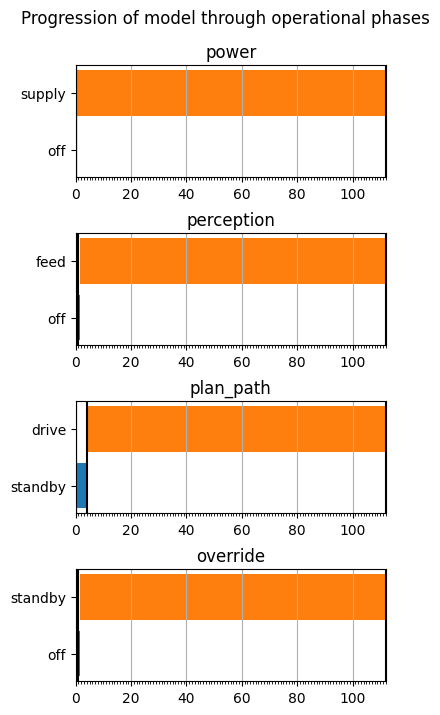
The PhaseMap for Power is here in power:
phases['power']
PhaseMap({'off': [0.0, 0.0], 'supply': [1.0, 112.0]}, {'off': {'off'}, 'supply': {'supply'}})
Which we can use to create a FaultSample which only samples the phases corresponding to the information given in Mode:
fs_pwr = FaultSample(fd_pwr, phasemap=phases['power'])
fs_pwr.add_fault_phases()
fs_pwr
FaultSample of scenarios:
 - rover_fxns_power_depleted_t0p0
 - rover_fxns_power_no_charge_t0p0
 - rover_fxns_power_short_t0p0
 - rover_fxns_power_depleted_t56p0
 - rover_fxns_power_no_charge_t56p0
 - rover_fxns_power_short_t56p0
If we look at the rate information, however:
fs_pwr.scenarios()
[SingleFaultScenario(sequence={0.0: Injection(faults={'rover.fxns.power': ['depleted']}, disturbances={})}, times=(0.0,), function='rover.fxns.power', fault='depleted', rate=1.0, name='rover_fxns_power_depleted_t0p0', time=0.0, phase='off'),
 SingleFaultScenario(sequence={0.0: Injection(faults={'rover.fxns.power': ['no_charge']}, disturbances={})}, times=(0.0,), function='rover.fxns.power', fault='no_charge', rate=1e-05, name='rover_fxns_power_no_charge_t0p0', time=0.0, phase='off'),
 SingleFaultScenario(sequence={0.0: Injection(faults={'rover.fxns.power': ['short']}, disturbances={})}, times=(0.0,), function='rover.fxns.power', fault='short', rate=0.0, name='rover_fxns_power_short_t0p0', time=0.0, phase='off'),
 SingleFaultScenario(sequence={56.0: Injection(faults={'rover.fxns.power': ['depleted']}, disturbances={})}, times=(56.0,), function='rover.fxns.power', fault='depleted', rate=1.0, name='rover_fxns_power_depleted_t56p0', time=56.0, phase='supply'),
 SingleFaultScenario(sequence={56.0: Injection(faults={'rover.fxns.power': ['no_charge']}, disturbances={})}, times=(56.0,), function='rover.fxns.power', fault='no_charge', rate=0.0, name='rover_fxns_power_no_charge_t56p0', time=56.0, phase='supply'),
 SingleFaultScenario(sequence={56.0: Injection(faults={'rover.fxns.power': ['short']}, disturbances={})}, times=(56.0,), function='rover.fxns.power', fault='short', rate=1e-05, name='rover_fxns_power_short_t56p0', time=56.0, phase='supply')]
The rate for scenarios outside the phases is zero!
We can remove these scenarios using FaultSample.prune_scenarios:
fs_pwr.prune_scenarios("rate", np.greater, 0.0)
fs_pwr
FaultSample of scenarios:
 - rover_fxns_power_depleted_t0p0
 - rover_fxns_power_no_charge_t0p0
 - rover_fxns_power_depleted_t56p0
 - rover_fxns_power_short_t56p0
fs_pwr.scenarios()
[SingleFaultScenario(sequence={0.0: Injection(faults={'rover.fxns.power': ['depleted']}, disturbances={})}, times=(0.0,), function='rover.fxns.power', fault='depleted', rate=1.0, name='rover_fxns_power_depleted_t0p0', time=0.0, phase='off'),
 SingleFaultScenario(sequence={0.0: Injection(faults={'rover.fxns.power': ['no_charge']}, disturbances={})}, times=(0.0,), function='rover.fxns.power', fault='no_charge', rate=1e-05, name='rover_fxns_power_no_charge_t0p0', time=0.0, phase='off'),
 SingleFaultScenario(sequence={56.0: Injection(faults={'rover.fxns.power': ['depleted']}, disturbances={})}, times=(56.0,), function='rover.fxns.power', fault='depleted', rate=1.0, name='rover_fxns_power_depleted_t56p0', time=56.0, phase='supply'),
 SingleFaultScenario(sequence={56.0: Injection(faults={'rover.fxns.power': ['short']}, disturbances={})}, times=(56.0,), function='rover.fxns.power', fault='short', rate=1e-05, name='rover_fxns_power_short_t56p0', time=56.0, phase='supply')]
As shown, now the only scenarios in the FaultSample are ones which have nonzero rate.
assert all([scen.rate > 0 for scen in fs_pwr.scenarios()])
To enable multiple samples to be generated for different faultdomains accross the model, we can use SampleApproach, e.g.:
phases
{'power': PhaseMap({'off': [0.0, 0.0], 'supply': [1.0, 112.0]}, {'off': {'off'}, 'supply': {'supply'}}),
 'perception': PhaseMap({'off': [0.0, 1.0], 'feed': [2.0, 112.0]}, {'off': {'off'}, 'feed': {'feed'}}),
 'plan_path': PhaseMap({'standby': [0.0, 4.0], 'drive': [5.0, 112.0]}, {'standby': {'standby'}, 'drive': {'drive'}}),
 'override': PhaseMap({'off': [0.0, 1.0], 'standby': [2.0, 112.0]}, {'off': {'off'}, 'standby': {'standby'}})}
sa = SampleApproach(Rover(), phasemaps=phases)
# adding fault domains
sa.add_faultdomain("drive", "fault", "drive", "custom")
sa.add_faultdomain("plan_path", "all_fxn_modes", "plan_path")
sa.add_faultdomain("power", "all_fxn_modes", "power")
sa.add_faultsample("drive", "fault_phases", "drive", phasemap="plan_path")
sa.add_faultsample("plan_path", "fault_phases", "plan_path", phasemap="plan_path")
sa.add_faultsample("power", "fault_phases", "power", phasemap="power")
sa.prune_scenarios()
sa
SampleApproach for rover with:
 faultdomains: drive, plan_path, power
 faultsamples: drive, plan_path, power
sa.scenarios()
[SingleFaultScenario(sequence={58.0: Injection(faults={'drive': ['custom']}, disturbances={})}, times=(58.0,), function='drive', fault='custom', rate=1.0, name='drive_custom_t58p0', time=58.0, phase='drive'),
 SingleFaultScenario(sequence={2.0: Injection(faults={'rover.fxns.plan_path': ['crash']}, disturbances={})}, times=(2.0,), function='rover.fxns.plan_path', fault='crash', rate=0.0001, name='rover_fxns_plan_path_crash_t2p0', time=2.0, phase='standby'),
 SingleFaultScenario(sequence={2.0: Injection(faults={'rover.fxns.plan_path': ['no_con']}, disturbances={})}, times=(2.0,), function='rover.fxns.plan_path', fault='no_con', rate=0.0001, name='rover_fxns_plan_path_no_con_t2p0', time=2.0, phase='standby'),
 SingleFaultScenario(sequence={58.0: Injection(faults={'rover.fxns.plan_path': ['crash']}, disturbances={})}, times=(58.0,), function='rover.fxns.plan_path', fault='crash', rate=0.0001, name='rover_fxns_plan_path_crash_t58p0', time=58.0, phase='drive'),
 SingleFaultScenario(sequence={58.0: Injection(faults={'rover.fxns.plan_path': ['no_con']}, disturbances={})}, times=(58.0,), function='rover.fxns.plan_path', fault='no_con', rate=0.0001, name='rover_fxns_plan_path_no_con_t58p0', time=58.0, phase='drive'),
 SingleFaultScenario(sequence={0.0: Injection(faults={'rover.fxns.power': ['depleted']}, disturbances={})}, times=(0.0,), function='rover.fxns.power', fault='depleted', rate=1.0, name='rover_fxns_power_depleted_t0p0', time=0.0, phase='off'),
 SingleFaultScenario(sequence={0.0: Injection(faults={'rover.fxns.power': ['no_charge']}, disturbances={})}, times=(0.0,), function='rover.fxns.power', fault='no_charge', rate=1e-05, name='rover_fxns_power_no_charge_t0p0', time=0.0, phase='off'),
 SingleFaultScenario(sequence={56.0: Injection(faults={'rover.fxns.power': ['depleted']}, disturbances={})}, times=(56.0,), function='rover.fxns.power', fault='depleted', rate=1.0, name='rover_fxns_power_depleted_t56p0', time=56.0, phase='supply'),
 SingleFaultScenario(sequence={56.0: Injection(faults={'rover.fxns.power': ['short']}, disturbances={})}, times=(56.0,), function='rover.fxns.power', fault='short', rate=1e-05, name='rover_fxns_power_short_t56p0', time=56.0, phase='supply')]
This is mostly useful when we would like to sample different functions in a model differently than others (e.g., using different phases), but still want to propagate the scenarios together as a part of a single sample.
Propagating Faults
Given the FaultSample approach, faults can then be propagated through the model to get results. Note that these faults can be sampled in parallel if desired using a user-provided pool (see the parallel pool tutorial in the \pump example folder).
res, hist = prop.fault_sample(Rover(), fs_pwr)
SCENARIOS COMPLETE: 100%|██████████| 4/4 [00:00<00:00, 10.00it/s]
fs_pwr.scenarios()
[SingleFaultScenario(sequence={0.0: Injection(faults={'rover.fxns.power': ['depleted']}, disturbances={})}, times=(0.0,), function='rover.fxns.power', fault='depleted', rate=1.0, name='rover_fxns_power_depleted_t0p0', time=0.0, phase='off'),
 SingleFaultScenario(sequence={0.0: Injection(faults={'rover.fxns.power': ['no_charge']}, disturbances={})}, times=(0.0,), function='rover.fxns.power', fault='no_charge', rate=1e-05, name='rover_fxns_power_no_charge_t0p0', time=0.0, phase='off'),
 SingleFaultScenario(sequence={56.0: Injection(faults={'rover.fxns.power': ['depleted']}, disturbances={})}, times=(56.0,), function='rover.fxns.power', fault='depleted', rate=1.0, name='rover_fxns_power_depleted_t56p0', time=56.0, phase='supply'),
 SingleFaultScenario(sequence={56.0: Injection(faults={'rover.fxns.power': ['short']}, disturbances={})}, times=(56.0,), function='rover.fxns.power', fault='short', rate=1e-05, name='rover_fxns_power_short_t56p0', time=56.0, phase='supply')]
hist.rover_fxns_power_short_t56p0.flows.pos.s.x
array([ 0.        ,  0.        ,  0.        ,  0.        ,  0.        ,
        0.26228971,  0.49976748,  0.75073622,  1.02156689,  1.32129469,
        1.64872275,  1.97931323,  2.28554745,  2.5617033 ,  2.81293761,
        3.05023699,  3.27790299,  3.50955358,  3.74782502,  4.00173726,
        4.27958216,  4.58909344,  4.92131254,  5.24511574,  5.53944945,
        5.80388536,  6.04976253,  6.28347644,  6.51647431,  6.75159711,
        6.99704083,  7.26107844,  7.55319773,  7.87591486,  8.20846606,
        8.51950465,  8.79935905,  9.05524795,  9.29420557,  9.52437137,
        9.75690271,  9.99541657, 10.24718399, 10.5213614 , 10.82691482,
       11.15775968, 11.48436846, 11.78261477, 12.05194732, 12.29896633,
       12.53412411, 12.76759447, 13.00158045, 13.24371735, 13.50429217,
       13.79153424, 14.11009375, 14.4433811 , 14.75940856, 15.04465136,
       15.30237525, 15.54407263, 15.7756063 , 16.00796687, 16.24490728,
       16.49506726, 16.76634091, 17.06780748, 17.39659755, 17.72559436,
       18.02745202, 18.29919904, 18.54970736, 18.78576416, 19.0201945 ,
       19.25406815, 19.49550135, 19.75267898, 20.03543446, 20.3502719 ,
       20.68350322, 21.00283298, 21.2912787 , 21.55318904, 21.79568028,
       22.02826326, 22.26081145, 22.4969189 , 22.74393521, 23.0114501 ,
       23.30883578, 23.63496159, 23.96603545, 24.27286793, 24.54935844,
       24.80104437, 25.0390264 , 25.26819146, 25.50091017, 25.74042655,
       25.99578368, 25.99578368])
hist.rover_fxns_power_short_t56p0.fxns.power.s.charge
array([100.   ,  99.99 ,  99.98 ,  99.8  ,  99.62 ,  99.44 ,  99.235,
        99.03 ,  98.825,  98.62 ,  98.415,  98.21 ,  98.005,  97.8  ,
        97.595,  97.39 ,  97.185,  96.98 ,  96.775,  96.57 ,  96.365,
        96.16 ,  95.955,  95.75 ,  95.545,  95.34 ,  95.135,  94.93 ,
        94.725,  94.52 ,  94.315,  94.11 ,  93.905,  93.7  ,  93.495,
        93.29 ,  93.085,  92.88 ,  92.675,  92.47 ,  92.265,  92.06 ,
        91.855,  91.65 ,  91.445,  91.24 ,  91.035,  90.83 ,  90.625,
        90.42 ,  90.215,  90.01 ,  89.805,  89.6  ,  89.395,  89.19 ,
        88.985,  86.935,  84.885,  82.835,  80.785,  78.735,  76.685,
        74.635,  72.585,  70.535,  68.485,  66.435,  64.385,  62.335,
        60.285,  58.235,  56.185,  54.135,  52.085,  50.035,  47.985,
        45.935,  43.885,  41.835,  39.785,  37.735,  35.685,  33.635,
        31.585,  29.535,  27.485,  25.435,  23.385,  21.335,  19.285,
        17.235,  15.185,  13.135,  11.085,   9.035,   6.985,   4.935,
         2.885,   0.835,   0.   ,   0.   ])
res
rover_fxns_power_dep                 1.0
rover_fxns_power_dep                   0
rover_fxns_power_dep                 1.0
rover_fxns_power_dep                   0
rover_fxns_power_dep                True
rover_fxns_power_dep               False
rover_fxns_power_dep                   1
rover_fxns_power_dep                   1
rover_fxns_power_dep   3.258651134742929
rover_fxns_power_dep 0.11859644458085598
rover_fxns_power_dep            array(1)
rover_fxns_power_depincomplete mission faulty
rover_fxns_power_dep  25.995783679666012
rover_fxns_power_dep  0.7019136572504056
rover_fxns_power_dep            array(2)
rover_fxns_power_no_               1e-05
rover_fxns_power_no_                   0
rover_fxns_power_no_                 1.0
rover_fxns_power_no_                   0
rover_fxns_power_no_                True
rover_fxns_power_no_               False
rover_fxns_power_no_                   1
rover_fxns_power_no_                   1
rover_fxns_power_no_   28.91724385770989
rover_fxns_power_no_                 0.0
rover_fxns_power_no_            array(1)
rover_fxns_power_no_incomplete mission faulty
rover_fxns_power_no_                 0.0
rover_fxns_power_no_                 0.0
rover_fxns_power_no_            array(2)
rover_fxns_power_dep                 1.0
rover_fxns_power_dep                   0
rover_fxns_power_dep                 1.0
rover_fxns_power_dep                   0
rover_fxns_power_dep                True
rover_fxns_power_dep                True
rover_fxns_power_dep                   1
rover_fxns_power_dep                   1
rover_fxns_power_dep                 0.0
rover_fxns_power_dep 0.11859644458085598
rover_fxns_power_dep            array(1)
rover_fxns_power_dep              faulty
rover_fxns_power_dep  29.254775331608617
rover_fxns_power_dep -0.7827640334587979
rover_fxns_power_dep            array(2)
rover_fxns_power_sho               1e-05
rover_fxns_power_sho                   0
rover_fxns_power_sho                 1.0
rover_fxns_power_sho                   0
rover_fxns_power_sho                True
rover_fxns_power_sho               False
rover_fxns_power_sho                   1
rover_fxns_power_sho                   1
rover_fxns_power_sho   3.258651134742929
rover_fxns_power_sho 0.11859644458085598
rover_fxns_power_sho            array(1)
rover_fxns_power_shoincomplete mission faulty
rover_fxns_power_sho  25.995783679666012
rover_fxns_power_sho  0.7019136572504056
rover_fxns_power_sho            array(2)
nominal.endclass.rate:               1.0
nominal.endclass.cost:                 0
nominal.endclass.prob:               1.0
nominal.endclass.expected_cost:        0
nominal.endclass.in_bound:          True
nominal.endclass.at_finish:         True
nominal.endclass.line_dist:            1
nominal.endclass.num_modes:            0
nominal.endclass.end_dist:           0.0
nominal.endclass.tot_deviation: 0.11859644458085598
nominal.endclass.faults:        array(0)
nominal.endclass.classification: nominal mission
nominal.endclass.end_x: 29.254775331608617
nominal.endclass.end_y: -0.7827640334587979
nominal.endclass.endpt:         array(2)
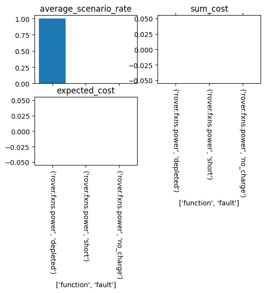
These responses can be visualized over the given faults:
fmea = FMEA(res, fs_pwr, metrics = ["end_dist", "line_dist", "tot_deviation"])
fmea.as_table()
| average_scenario_rate | sum_cost | expected_cost | ||
|---|---|---|---|---|
| rover.fxns.power | depleted | 1.00000 | 0 | 0.0 |
| short | 0.00001 | 0 | 0.0 | |
| no_charge | 0.00001 | 0 | 0.0 |
fmea.as_plots(cols=2)
(<Figure size 600x400 with 4 Axes>,
 array([<Axes: title={'center': 'average_scenario_rate'}>,
        <Axes: title={'center': 'sum_cost'}, xlabel="['function', 'fault']">,
        <Axes: title={'center': 'expected_cost'}, xlabel="['function', 'fault']">,
        <Axes: >], dtype=object))
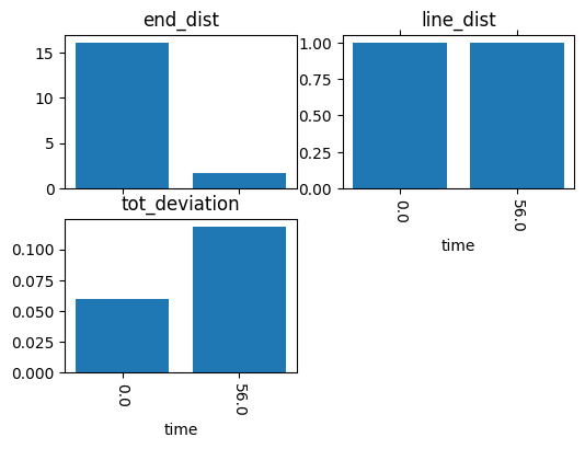
Or over time/any other variable:
comp = Comparison(res, fs_pwr, metrics = ["end_dist", "line_dist", "tot_deviation"], factors =['time'])
comp.as_table()
| end_dist | line_dist | tot_deviation | |
|---|---|---|---|
| 56.0 | 1.629326 | 1.0 | 0.118596 |
| 0.0 | 16.087947 | 1.0 | 0.059298 |
comp.as_plots(cols=2)
(<Figure size 600x400 with 4 Axes>,
 array([<Axes: title={'center': 'end_dist'}>,
        <Axes: title={'center': 'line_dist'}, xlabel='time'>,
        <Axes: title={'center': 'tot_deviation'}, xlabel='time'>, <Axes: >],
       dtype=object))
Parameteric Fault Samples
Faults defined as fields can be instantiated and sampled parametrically. This enables the representation of different fault paramters. An example of a fault parameter would be depletion charge, represented below:
print(inspect.getsource(PowerMode))
class PowerMode(Mode):
    """
    Possible modes for Power function.

    Modes
    -------
    no_charge : Fault
        Battery is out of charge.
    short: Fault
        There is a short.
    depletion: Fault
        The battery is depleted to a given percent
    supply: Mode
        supply power
    charge: Mode
        charge battery
    standby: Mode
        power supply is in stand by
    off: Mode
        power supply is off
    """

    fault_no_charge = (1e-5, 100, (("off", 1.0),))
    fault_short = (1e-5, 100, (("supply", 1.0),))
    fault_depleted: dict = {'disturbances': {'s.charge': 20.0}}
    opermodes = ("supply", "charge", "off")
    mode: str = "off"
    exclusive = True
mdl = Rover()
mdl.fxns['power'].m.get_fault('depleted')
Fault(prob=1.0, cost=0.0, phases=(), disturbances={'s.charge': 20.0}, units='sim')
This fault can be readily changed as a parameter of the Power class:
p = Power(m={'fault_depleted': {'disturbances': {'s.charge': 13.0 }}})
p
power Power
- PowerState(charge=100.0, power=0.0)
- PowerMode(mode=off, faults=set())
p.m.get_fault('depleted')
Fault(prob=1.0, cost=0.0, phases=(), disturbances={'s.charge': 13.0}, units='sim')
It can also be sampled at different levels in a FaultSample by adding the same fault at multiple levels:
fd_dep = FaultDomain(mdl)
fd_dep.add_fault('power', 'depleted', ind="5", disturbances={'s.charge': 5})
fd_dep.add_fault('power', 'depleted', ind="15", disturbances={'s.charge': 15})
fd_dep.add_fault('power', 'depleted', ind="0", disturbances={'s.charge': 0})
fd_dep
FaultDomain with faults:
 -('power', 'depleted', '5')
 -('power', 'depleted', '15')
 -('power', 'depleted', '0')
These faults can then be sampled as normal. For example, below we sample the modes at two fault times:
fs_dep = FaultSample(fd_dep)
fs_dep.add_fault_times([5, 10])
fs_dep
FaultSample of scenarios:
 - power_depleted_5_t5
 - power_depleted_5_t10
 - power_depleted_15_t5
 - power_depleted_15_t10
 - power_depleted_0_t5
 - power_depleted_0_t10
res, hist = prop.fault_sample(mdl, fs_dep)
SCENARIOS COMPLETE: 100%|██████████| 6/6 [00:00<00:00, 17.33it/s]
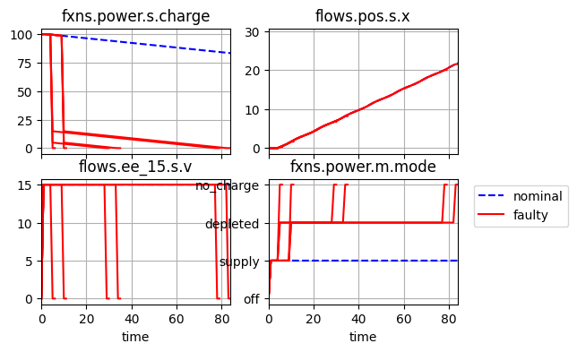
You can see the effects of the different types of faults below. As shown, the battery charge is lowered to three different levels at three different times, leading to the simulation ending at different times as the rover loses charge:
hist.plot_line('fxns.power.s.charge', 'flows.pos.s.x', 'flows.ee_15.s.v', 'fxns.power.m.mode')
(<Figure size 600x400 with 4 Axes>,
 array([<Axes: title={'center': 'fxns.power.s.charge'}, xlabel=' '>,
        <Axes: title={'center': 'flows.pos.s.x'}, xlabel=' '>,
        <Axes: title={'center': 'flows.ee_15.s.v'}, xlabel='time'>,
        <Axes: title={'center': 'fxns.power.m.mode'}, xlabel='time'>],
       dtype=object))
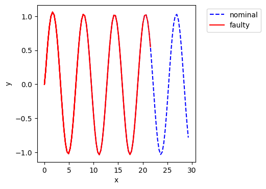
hist.plot_trajectories('pos.s.x', 'pos.s.y')
(<Figure size 400x400 with 1 Axes>, <Axes: xlabel='x', ylabel='y'>)
