Defining and Visualizing fmdtools Model Structures
To ensure that a simulation meets the intent of a modeller, it is important to carefully define the structure of the model and run order. This notebook will demonstrate fmdtools’ interfaces both for setting up model structures and for fault visualization.
NOTE: For some of these visualizations to display properly without re-running code, use File -> Trust Notebook.
Copyright © 2024, United States Government, as represented by the Administrator of the National Aeronautics and Space Administration. All rights reserved.
The “"Fault Model Design tools - fmdtools version 2"” software is licensed under the Apache License, Version 2.0 (the "License"); you may not use this file except in compliance with the License. You may obtain a copy of the License at http://www.apache.org/licenses/LICENSE-2.0.
Unless required by applicable law or agreed to in writing, software distributed under the License is distributed on an "AS IS" BASIS, WITHOUT WARRANTIES OR CONDITIONS OF ANY KIND, either express or implied. See the License for the specific language governing permissions and limitations under the License.
from fmdtools.define.architecture.function import FunctionArchitecture
from fmdtools.define.block.function import Function
from fmdtools.define.block.component import Component
import fmdtools.sim.propagate as prop
Basics
An fmdtools model is made up of functions–model structures with behavioral methods and internal states–and flows–data relationships between functions. These functions and flows are defined in python classes and thus may be instantiated multiple times in a model to create multi-component models with complex interactions. The structure of these model classes is shown below:
Creating a model thus involves:
defining the function and flow classes defining the behavior of the model in the model module
defining the specific structure for the model: function and flow objects (instantiations of functions) and their relationships.
Model structure visualization is performed in the analyze.graph.architecture.FunctionArchitectureGraph class and its sub-classes.
from fmdtools.define.architecture.function import FunctionArchitectureGraph
help(FunctionArchitectureGraph)
Help on class FunctionArchitectureGraph in module fmdtools.define.architecture.function:
class FunctionArchitectureGraph(fmdtools.define.architecture.base.ArchitectureGraph)
| FunctionArchitectureGraph(mdl, get_states=True, time=0.0, check_info=False, **kwargs)
|
| Graph of FunctionArchitecture, where both functions and flows are nodes.
|
| If get_states option is used on instantiation, a `states` dict is associated
| with the edges/nodes which can then be used to visualize function/flow attributes.
|
| Examples
| --------
| >>> efa = FunctionArchitectureGraph(ExFxnArch())
| >>> efa.g.nodes()
| NodeView(('exfxnarch.flows.exf', 'exfxnarch.fxns.ex_fxn', 'exfxnarch.fxns.ex_fxn2'))
| >>> efa.g.edges()
| OutEdgeView([('exfxnarch.fxns.ex_fxn', 'exfxnarch.flows.exf'), ('exfxnarch.fxns.ex_fxn2', 'exfxnarch.flows.exf')])
|
| Method resolution order:
| FunctionArchitectureGraph
| fmdtools.define.architecture.base.ArchitectureGraph
| fmdtools.analyze.graph.model.ExtModelGraph
| fmdtools.analyze.graph.model.ModelGraph
| fmdtools.analyze.graph.base.Graph
| builtins.object
|
| Methods defined here:
|
| draw_graphviz(self, layout='twopi', overlap='voronoi', **kwargs)
| Draw the graph using pygraphviz for publication-quality figures.
|
| Note that the style may not match one-to-one with the defined none/edge styles.
|
| Parameters
| ----------
| disp : bool
| Whether to display the plot. The default is True.
| saveas : str
| File to save the plot as. The default is '' (which doesn't save the plot').
| **kwargs : kwargs
| Arguments for various supporting functions:
| (set_pos, set_edge_styles, set_edge_labels, set_node_styles,
| set_node_labels, etc)
| Can also provide kwargs for Digraph() initialization.
|
| Returns
| -------
| dot : PyGraphviz DiGraph
| Graph object corresponding to the figure.
|
| gen_func_arch_graph(self, mdl)
| Generate function architecture graph.
|
| get_dynamicnodes(self, mdl)
| Get dynamic node information for set_exec_order.
|
| get_multi_edges(self, graph, subedges)
| Attach functions/flows (subedges arg) to edges.
|
| Parameters
| ----------
| graph: networkx graph
| Graph of model to represent
| subedges : list
| nodes from the full graph which will become edges in the subgraph
| (e.g., individual flows)
|
| Returns
| -------
| flows : dict
| Dictionary of edges with keys representing each sub-attribute of the
| edge (e.g., flows)
|
| get_staticnodes(self, mdl)
| Get static node information for set_exec_order.
|
| set_exec_order(self, mdl, static={}, dynamic={}, next_edges={}, label_order=True, label_tstep=True)
| Overlay FunctionArchitectureGraph execution order data on graph structure.
|
| Parameters
| ----------
| mdl : Model
| Model to plot the execution order of.
| static : dict/False, optional
| kwargs to overwrite the default style for functions/flows in the static
| execution step.
| If False, static functions are not differentiated. The default is {}.
| dynamic : dict/False, optional
| kwargs to overwrite the default style for functions/flows in the dynamic
| execution step.
| If False, dynamic functions are not differentiated. The default is {}.
| next_edges : dict
| kwargs to overwrite the default style for edges indicating the flow order.
| If False, these edges are not added. the default is {}.
| label_order : bool, optional
| Whether to label execution order (with a number on each node).
| The default is True.
| label_tstep : bool, optional
| Whether to label each timestep (with a number in the subtitle).
| The default is True.
|
| set_flow_nodestates(self, mdl, with_root=True)
| Attach attributes to Graph notes corresponding to flow states.
|
| Parameters
| ----------
| mdl: Model
| Model to represent
|
| set_fxn_nodestates(self, mdl, with_root=True)
| Attach attributes to Graph corresponding to function states.
|
| Parameters
| ----------
| mdl: Model
| Model to represent
|
| ----------------------------------------------------------------------
| Methods inherited from fmdtools.define.architecture.base.ArchitectureGraph:
|
| draw_from(self, *args, rem_ind=2, **kwargs)
| Set from a history (removes prefixes so it works at top level).
|
| nx_from_obj(self, mdl, with_root=False, **kwargs)
| Generate the networkx.graph object corresponding to the model.
|
| Parameters
| ----------
| mdl: FunctionArchitecture
| Model to create the graph representation of
|
| Returns
| -------
| g : networkx.Graph
| networkx.Graph representation of model functions and flows
| (along with their attributes)
|
| set_nx_states(self, mdl, **kwargs)
| Set the states of the graph.
|
| ----------------------------------------------------------------------
| Methods inherited from fmdtools.analyze.graph.model.ExtModelGraph:
|
| __init__(self, mdl, get_states=True, time=0.0, check_info=False, **kwargs)
| Generate the FunctionArchitectureGraph corresponding to a given Model.
|
| Parameters
| ----------
| mdl : object
| fmdtools object to represent graphically
| get_states : bool, optional
| Whether to copy states to the node/edge 'states' property.
| The default is True.
| time: float
| Time model is run at (to execute indicators at). Default is 0.0
| **kwargs : kwargs
| (placeholder for kwargs)
|
| ----------------------------------------------------------------------
| Methods inherited from fmdtools.analyze.graph.model.ModelGraph:
|
| animate(self, history, times='all', figsize=(6, 4), **kwargs)
| Successively animate a plot using Graph.draw_from.
|
| Parameters
| ----------
| history : History
| History with faulty and nominal states
| times : list, optional
| List of times to animate over. The default is 'all'
| figsize : tuple, optional
| Size for the figure. The default is (6,4)
| **kwargs : kwargs
|
| Returns
| -------
| ani : matplotlib.animation.FuncAnimation
| Animation object with the given frames
|
| draw_graphviz_from(self, time, history=, **kwargs)
| Draws the graph with degraded/fault data at a given time.
|
| Parameters
| ----------
| time : int
| Time to draw the graph (in the history)
| history : History, optional
| History with nominal and faulty history. The default is History().
| **kwargs : **kwargs
| arguments for Graph.draw
|
| Returns
| -------
| dot : graphvis graph
| Graph drawn with attributes at the given time.
|
| get_nodes(self, rem_ind=0)
| Get nodes (with shortened names if needed).
|
| set_degraded(self, other)
| Set 'degraded' state in networkx graph.
|
| Uses difference between states with another Graph object.
|
| Parameters
| ----------
| other : Graph
| (assumed nominal) Graph to compare to
|
| set_from(self, time, history=, rem_ind=0)
| Set ModelGraph faulty/degraded attributes from a given history.
|
| set_resgraph(self, other=False)
| Process results for results graphs (show faults and degradations).
|
| Parameters
| ----------
| other : Graph, optional
| Graph to compare with (for degradations). The default is False.
|
| ----------------------------------------------------------------------
| Methods inherited from fmdtools.analyze.graph.base.Graph:
|
| add_node_groups(self, **node_groups)
| Create arbitrary groups of nodes to displayed with different styles.
|
| Parameters
| ----------
| **node_groups : iterable
| nodes in groups. see example.
|
| Examples
| --------
| >>> graph = Graph(ex_nxgraph)
| >>> graph.add_node_groups(group1=('function_a', 'function_b'), group2=('function_c',))
| >>> graph.set_node_styles(group={'group1': {'nx_node_color':'green'}, 'group2': {'nx_node_color':'red'}})
| >>> fig, ax = graph.draw()
|
| would show two different groups of nodes, one with green nodes, and the other
| with red nodes
|
| calc_aspl(self)
| Compute average shortest path length of the graph.
|
| Returns
| -------
| aspl: float
| Average shortest path length
|
| calc_modularity(self)
| Compute network modularity of the graph.
|
| Returns
| -------
| modularity : Modularity
|
| calc_node_betweenness(self)
| Calculate betweenness for nodes.
|
| calc_node_closeness(self)
| Calculate closeness dict for nodes.
|
| calc_node_degree(self)
| Calculate degree dict for nodes.
|
| calc_node_eigenvector(self)
| Calculate eigenvector centrality for nodes.
|
| calc_robustness_coefficient(self, trials=100, seed=False)
| Compute robustness coefficient of graph representation of model mdl.
|
| Parameters
| ----------
| trials : int
| number of times to run robustness coefficient algorithm
| (result is averaged over all trials)
| seed : int
| optional seed to instantiate test with
|
| Returns
| -------
| RC : robustness coefficient
|
| check_type_info(self)
| Check that nodes and edges have type data.
|
| compare_with(self, other_graph)
| Compare this graph with another graph to identify structural differences.
|
| Useful for comparing different model variants, design alternatives, or
| tracking how model structure evolves across versions.
|
| Parameters
| ----------
| other_graph : Graph
| Another Graph object to compare with.
|
| Returns
| -------
| dict
| Comparison results including:
| - nodes_added : set
| Nodes present in other_graph but not in this graph
| - nodes_removed : set
| Nodes present in this graph but not in other_graph
| - edges_added : set
| Edges present in other_graph but not in this graph
| - edges_removed : set
| Edges present in this graph but not in other_graph
| - structure_similarity : float
| Jaccard similarity coefficient for overall structure (0-1)
| - summary_this : dict
| Summary statistics for this graph
| - summary_other : dict
| Summary statistics for the other graph
|
| Examples
| --------
| >>> from examples.pump.ex_pump import Pump
| >>> from examples.rover.rover_model import Rover
| >>> from fmdtools.define.architecture.function import FunctionArchitectureGraph
| >>> pump_graph = FunctionArchitectureGraph(Pump())
| >>> rover_graph = FunctionArchitectureGraph(Rover())
| >>> comparison = pump_graph.compare_with(rover_graph)
| >>> len(comparison['nodes_added']) > 0
| True
|
| draw(self, figsize=(12, 10), title='', fig=False, ax=False, withlegend=True, legend_bbox=(1, 0.5), legend_loc='center left', legend_labelspacing=2, legend_borderpad=1, saveas='', **kwargs)
| Draw a graph with given styles corresponding to the node/edge properties.
|
| Parameters
| ----------
| figsize : tuple, optional
| Size for the figure (plt.figure arg). The default is (12,10).
| title : str, optional
| Title for the plot. The default is "".
| fig : bool, optional
| matplotlib figure to project on (if provided). The default is False.
| ax : bool, optional
| matplotlib axis to plot on (if provided). The default is False.
| withlegend : bool, optional
| Whether to include a legend. The default is True.
| legend_bbox : tuple, optional
| bbox to anchor the legend to. The default is (1,0.5), which places legend
| on the right.
| legend_loc : str, optional
| loc argument for plt.legend. The default is "center left".
| legend_labelspacing : float, optional
| labelspacing argument for plt.legend. the default is 2.
| legend_borderpad : str, optional
| borderpad argument for plt.legend. the default is 1.
| saveas : str, optional
| file to save as (if provided).
| **kwargs : kwargs
| Arguments for various supporting functions:
| (set_pos, set_edge_styles, set_edge_labels, set_node_styles,
| set_node_labels, etc)
|
| Returns
| -------
| fig : matplotlib figure
| matplotlib figure to draw
| ax : matplotlib axis
| Ax in the figure
|
| draw_drawio(self, saveas='', **kwargs)
| Generate DrawIO diagram using existing graph structure and positions.
|
| Parameters
| ----------
| saveas : str, optional
| File path to save the DrawIO XML. If empty, returns XML content.
| **kwargs : dict
| Additional arguments for graph styling and positioning.
|
| Returns
| -------
| xml_content : str
| DrawIO XML content.
|
| Examples
| --------
| >>> graph = Graph(ex_nxgraph)
| >>> xml_content = graph.draw_drawio() # Get XML content
| >>> xml_content = graph.draw_drawio("graph.drawio") # Save to file
|
| find_bridging_nodes(self)
| Determine bridging nodes in a graph representation of model mdl.
|
| Returns
| -------
| bridgingNodes : list of bridging nodes
|
| find_high_degree_nodes(self, p=90)
| Determine highest degree nodes, up to percentile p, in graph.
|
| Parameters
| ----------
| p : int (optional)
| percentile of degrees to return, between 0 and 100
|
| Returns
| -------
| highDegreeNodes : list of high degree nodes in format (node,degree)
|
| get_node_percentiles(self, metric='betweenness', quartiles=[0, 25, 50, 75])
| Get the quartiles of a node for a given metric.
|
| Parameters
| ----------
| metric : str or callable, optional
| If str: Predefined centrality (calls calc_strname). Options:
| - 'betweenness': Betweenness centrality (via NetworkX)
| - 'closeness': Closeness centrality (via NetworkX)
| - 'eigenvector': Eigenvector centrality (via NetworkX)
| - 'degree': Degree centrality
| If callable: Function that accepts self.g and returns dict of {node: value}.
| Default is 'betweenness'.
| quartiles : list, optional
| Percentile boundaries for grouping nodes. Default is [0, 25, 50, 75].
| Must have length >= 2.
|
| Returns
| -------
| groups : dict
| Dict of nodes in each quartile.
|
| Examples
| --------
| >>> graph = Graph(ex_nxgraph)
| >>> graph.get_node_percentiles("degree")
| {0: ['external_signals', 'external_energy_in', 'external_material_in', 'external_material_out', 'external_energy_out'], 25: [], 50: ['control_signal', 'internal_energy'], 75: ['function_a', 'function_b', 'function_c']}
|
| move_nodes(self, **kwargs)
| Set the position of nodes for plots in analyze.graph using a graphical tool.
|
| Note: make sure matplotlib is set to plot in an external window
| (e.g., using '%matplotlib qt)
|
| Parameters
| ----------
| **kwargs : kwargs
| keyword arguments for graph.draw
|
| Returns
| -------
| p : GraphIterator
| Graph Iterator (in analyze.Graph)
|
| plot_bridging_nodes(self, title='bridging nodes', node_kwargs={'nx_node_color': 'red', 'gv_fillcolor': 'red'}, **kwargs)
| Plot bridging nodes using self.draw().
|
| Parameters
| ----------
| title : str, optional
| Title for the plot. The default is 'bridging nodes'.
| node_kwargs : dict, optional
| Non-default fields for NodeStyle
| **kwargs : kwargs
| kwargs for Graph.draw
|
| Returns
| -------
| fig : matplotlib figure
| Figure
|
| plot_degree_dist(self)
| Plot degree distribution of graph representation of model mdl.
|
| Returns
| -------
| fig : matplotlib figure
| plot of distribution
|
| plot_high_degree_nodes(self, p=90, title='', node_kwargs={'nx_node_color': 'red', 'gv_fillcolor': 'red'}, **kwargs)
| Plot high-degree nodes using self.draw().
|
| Parameters
| ----------
| p : int (optional)
| percentile of degrees to return, between 0 and 100
| title : str, optional
| Title for the plot. The default is 'High Degree Nodes'.
| node_kwargs : dict : kwargs to overwrite the default NodeStyle
| **kwargs : kwargs
| kwargs for Graph.draw
|
| Returns
| -------
| fig : matplotlib figure
| Figure
|
| plot_node_percentiles(self, metric='betweenness', title='', colormap=<matplotlib.colors.LinearSegmentedColormap object at 0x000002A1FF8C2AD0>, quartiles=[0, 25, 50, 75], quartile_names={}, quartile_styles={}, **kwargs)
| Plot nodes colored by a centrality or custom metric.
|
| Visualizes the graph with nodes grouped by their metric scores into
| quartiles. Supports both predefined centrality metrics and custom
| metric functions.
|
| Parameters
| ----------
| title : str, optional
| Plot title. If empty, generates title from metric name.
| colormap : matplotlib colormap, optional
| Matplotlib colormap object for coloring nodes. plt.cm.coolwarm.
| quartile_names : dict, optional
| Names for quartile labels. Default is {}, which is just the numbers.
| quartile_styles : dict, optional
| Custom styles for each quartile group. Keys are quartile indices (0, 1, 2, 3),
| values are style dicts with 'nx_node_color' and/or 'gv_fillcolor'.
| Example: {0: {'nx_node_color': 'red'}, 3: {'nx_node_color': 'blue'}}
| **kwargs : dict
| Additional keyword arguments passed to Graph.draw().
|
| Returns
| -------
| fig : matplotlib.figure.Figure
| The figure containing the plot.
|
| Examples
| --------
| >>> # Using predefined metric
| >>> graph = Graph(ex_nxgraph)
| >>> graph.set_pos(auto='spring')
| >>> fig = graph.plot_node_percentiles(metric='betweenness')
| >>>
| >>> # Using custom metric function
| >>> import networkx as nx
| >>> custom_metric = lambda g: nx.pagerank(g)
| >>> fig = graph.plot_node_percentiles(metric=custom_metric, title='PageRank')
| >>>
| >>> # Using custom quartiles and styles
| >>> quartile_styles = {"0": {'nx_node_color': 'orange'},
| ... "30": {'nx_node_color': 'green'}}
| >>> fig = graph.plot_node_percentiles(metric='degree', quartiles=[0, 30, 60, 90],
| ... quartile_styles=quartile_styles)
|
| set_edge_labels(self, title='edgetype', title2='', subtext='states', **edge_label_styles)
| Create labels using Labels.from_iterator for the edges in the graph.
|
| Parameters
| ----------
| title : str, optional
| property to get for title text. The default is 'id'.
| title2 : str, optional
| property to get for title text after the colon. The default is ''.
| subtext : str, optional
| property to get for the subtext. The default is 'states'.
| **edge_label_styles : dict
| LabelStyle arguments to overwrite.
|
| set_edge_styles(self, edgetype={}, **edge_styles)
| Set self.edge_styles and self.edge_groups given the provided edge styles.
|
| Parameters
| ----------
| edgetype : dict, optional
| kwargs to EdgeStyle for the given node type (e.g., containment, etc).
| **edge_styles : dict, optional
| Dictionary of tags, labels, and styles for the edges that overwrite the
| default. Has structure {tag:{label:kwargs}}, where kwargs are the keyword
| arguments to nx.draw_networkx_edges. The default is {"label":{}}.
|
| set_heatmap(self, heatmap, cmap=<matplotlib.colors.LinearSegmentedColormap object at 0x000002A1FF8C2AD0>, default_color_val=0.0, vmin=None, vmax=None)
| Set the association and plotting of a heatmap on a graph.
|
| Parameters
| ----------
| heatmap : dict/result
| dict/result with keys corresponding to the nodes and values in the range
| of a heatmap (0-1)
| cmap : mpl.Colormap, optional
| Colormap to use for the heatmap. The default is plt.cm.coolwarm.
| default_color_val : float, optional
| Value to use if a node is not in the heatmap dict. The default is 0.0.
| vmin : float
| Minimum value for the heatmap. Default is None, which sets it to the minimum
| value of the heatmap.
| vmax : float
| Maximum value for the heatmap. Default is None, which sets it to the maximum
| value of the heatmap.
|
| Examples
| --------
| The below should draw function a red, function b blue, function c pink, and all
| else grey:
| >>> graph = Graph(ex_nxgraph)
| >>> graph.set_heatmap({'function_a': 1.0, 'function_b': 0.0, 'function_c': 0.75}, default_color_val=0.5)
| >>> fig, ax = graph.draw()
|
| set_node_labels(self, title='shortname', title2='', subtext='', **node_label_styles)
| Create labels using Labels.from_iterator for the nodes in the graph.
|
| Parameters
| ----------
| title : str, optional
| Property to get for title text. The default is 'id'.
| title2 : str, optional
| Property to get for title text after the colon. The default is ''.
| subtext : str, optional
| property to get for the subtext. The default is ''.
| node_label_styles : dict
| LabelStyle arguments to overwrite.
|
| set_node_styles(self, nodetype={}, **node_styles)
| Set self.node_styles and self.edge_groups given the provided node styles.
|
| Parameters
| ----------
| nodetype : dict, optional
| kwargs to NodeStyle for the given node type (e.g., Block, Flow, etc).
| **node_styles : dict, optional
| Dictionary of tags, labels, and style kwargs for the nodes that overwrite
| the default. Has structure {tag:{label:kwargs}}, where kwargs are the
| keyword arguments to nx.draw_networkx_nodes. The default is {"label":{}}.
|
| set_pos(self, auto=True, overwrite=True, **pos)
| Set graph positions to given positions, (automatically or manually).
|
| Parameters
| ----------
| auto : str, optional
| Whether to auto-layout the node position. The default is True. If a string
| is provided, calls method_layout, where method is the string provided
| overwrite : bool, optional
| Whether to overwrite the existing pos. Default is True.
| **pos : nodename=(x,y)
| Positions of nodes to set. Otherwise updates to the auto-layout or (0.5,0.5)
|
| set_properties(self, **kwargs)
| Set properties using kwargs where there is a given set_kwarg command.
|
| sff_model(self, endtime=5, pi=0.1, pr=0.1, num_trials=100, start_node='random', error_bar_option='off')
| Susceptible-fix-fail model.
|
| Parameters
| ----------
| endtime: int
| simulation end time
| pi : float
| infection (failure spread) rate
| pr : float
| recovery (fix) rate
| num_trials : int
| number of times to run the epidemic model, default is 100
| error_bar_option : str
| option for plotting error bars (first to third quartile), default is off
| start_node : str
| start node to use in the trial. default is 'random'
|
| Returns
| -------
| fig: plot of susc, fail, and fix nodes over time
|
| summary(self)
| Generate a summary dictionary of key graph metrics.
|
| Provides a quick overview of graph structure and properties useful for
| model documentation, comparison, and resilience analysis.
|
| Returns
| -------
| dict
| Summary statistics including:
| - num_nodes : int
| Number of nodes in the graph
| - num_edges : int
| Number of edges in the graph
| - density : float
| Graph density (ratio of actual to possible edges)
| - is_connected : bool
| Whether the graph is connected (for directed graphs, this checks
| weak connectivity)
| - num_components : int
| Number of connected components (weakly connected for directed graphs)
| - avg_degree : float
| Average node degree
| - aspl : float or None
| Average shortest path length (only if graph is connected, None otherwise)
| - modularity : float
| Network modularity score (measures strength of division into communities)
|
| Examples
| --------
| >>> graph = Graph(ex_nxgraph)
| >>> summary = graph.summary()
| >>> summary['num_nodes']
| 10
| >>> summary['num_edges']
| 12
|
| ----------------------------------------------------------------------
| Data descriptors inherited from fmdtools.analyze.graph.base.Graph:
|
| __dict__
| dictionary for instance variables
|
| __weakref__
| list of weak references to the object
The main function used for displaying model structure is draw()
help(FunctionArchitectureGraph.draw)
Help on function draw in module fmdtools.analyze.graph.base:
draw(self, figsize=(12, 10), title='', fig=False, ax=False, withlegend=True, legend_bbox=(1, 0.5), legend_loc='center left', legend_labelspacing=2, legend_borderpad=1, saveas='', **kwargs)
Draw a graph with given styles corresponding to the node/edge properties.
Parameters
----------
figsize : tuple, optional
Size for the figure (plt.figure arg). The default is (12,10).
title : str, optional
Title for the plot. The default is "".
fig : bool, optional
matplotlib figure to project on (if provided). The default is False.
ax : bool, optional
matplotlib axis to plot on (if provided). The default is False.
withlegend : bool, optional
Whether to include a legend. The default is True.
legend_bbox : tuple, optional
bbox to anchor the legend to. The default is (1,0.5), which places legend
on the right.
legend_loc : str, optional
loc argument for plt.legend. The default is "center left".
legend_labelspacing : float, optional
labelspacing argument for plt.legend. the default is 2.
legend_borderpad : str, optional
borderpad argument for plt.legend. the default is 1.
saveas : str, optional
file to save as (if provided).
**kwargs : kwargs
Arguments for various supporting functions:
(set_pos, set_edge_styles, set_edge_labels, set_node_styles,
set_node_labels, etc)
Returns
-------
fig : matplotlib figure
matplotlib figure to draw
ax : matplotlib axis
Ax in the figure
However, these relationships only define the structure of the model–for the model to simulate correctly and efficiently, the run order of fuctions additionally must be defined.
Each timestep of a model simulation can be broken down into two steps:
Dynamic Propagation Step: In the dynamic propagation step, the time-based behaviors (e.g. accumulations, movement, etc.) are each run once in a specified order. These steps are generally quicker to execute because each behavior is only run once and the flows do not need to be tracked to determine which behaviors to execute next. This step is run first at each time-step of the model.
Static Propagation Step: In the static propagation step, behaviors are propagated between functions iteratively until the state of the model converges to a single value. This may require an update of multiple function behaviors until there are no more new behaviors to run. Thus, static behaviors should be ‘’timeless’’ (always give the same output for the same input) and convergent (behaviors in each function should not change each other ad infinitum). This step is run second at each time-step of the model.
With these different behaviors, one can express a range of different types of models:
static models where only only one timestep is run, where fault scenarios show the immediate propagation of faults through the system.
dynamic models where a number of timesteps are run (but behaviors are only run once).
hybrid models where dynamic behaviors are run once and then a static propagation step is performed at each time-step.
The main interfaces/functions involved in defining run order are:
Function.static_behavior(self), which define function behaviors which occur during the static propagation step.Function.dynamic_behavior(self), which defines function behaviors during the dynamic propagation step.FunctionArchitecture.add_fxn(), which when used successively for each function specifies that those functions run in the order they are added.
The overall static/dynamic propagation steps of the model can then be visualized using ModelGraph.set_exec_order successively with ModelGraph.draw().
help(FunctionArchitectureGraph.set_exec_order)
Help on function set_exec_order in module fmdtools.define.architecture.function:
set_exec_order(self, mdl, static={}, dynamic={}, next_edges={}, label_order=True, label_tstep=True)
Overlay FunctionArchitectureGraph execution order data on graph structure.
Parameters
----------
mdl : Model
Model to plot the execution order of.
static : dict/False, optional
kwargs to overwrite the default style for functions/flows in the static
execution step.
If False, static functions are not differentiated. The default is {}.
dynamic : dict/False, optional
kwargs to overwrite the default style for functions/flows in the dynamic
execution step.
If False, dynamic functions are not differentiated. The default is {}.
next_edges : dict
kwargs to overwrite the default style for edges indicating the flow order.
If False, these edges are not added. the default is {}.
label_order : bool, optional
Whether to label execution order (with a number on each node).
The default is True.
label_tstep : bool, optional
Whether to label each timestep (with a number in the subtitle).
The default is True.
The next sections will demonstrate these functions using a simple hybrid model.
Model Setup
Consider the following (highly simplified) rover electrical/navigation model. We can define the functions of this rover using the classes:
from fmdtools.define.container.state import State
from fmdtools.define.flow.base import Flow
from fmdtools.define.container.mode import Mode
class ControlState(State):
power: float=0.0
vel: float=0.0
class Control(Flow):
container_s = ControlState
class ControlRoverMode(Mode):
fault_no_con = (1e-4, 200)
opermodes = ('drive', 'standby')
mode : str='standby'
class ControlRover(Function):
container_m = ControlRoverMode
flow_control = Control
def dynamic_behavior(self):
if not self.m.in_mode('no_con'):
if self.t.time == 5: self.m.set_mode('drive')
if self.t.time == 50: self.m.set_mode('standby')
if self.m.in_mode('drive'):
self.control.s.power = 1.0
self.control.s.vel = 1.0
elif self.m.in_mode('standby'):
self.control.s.vel = 0.0
self.control.s.power=0.0
This function uses dynamic_behavior() to define the dynamic behavior of going through different modes depending on what model time it is. While this could also be entered in as a static behavior, because none of the defined behaviors themselves result from external inputs, there is no reason to.
class ForceState(State):
transfer: float=1.0
magnitude: float=1.0
class Force(Flow):
container_s = ForceState
class EEState(State):
v: float=0.0
a: float=0.0
class EE(Flow):
container_s = EEState
class GroundState(State):
x: float=0.0
class Ground(Flow):
container_s = GroundState
class MoveRoverMode(Mode):
fault_mech_loss = (1.0,)
fault_short = (1.0,)
fault_elec_open = (1.0,)
class MoveRoverState(State):
power: float=0.0
class MoveRover(Function):
container_s = MoveRoverState
container_m = MoveRoverMode
flow_ee = EE
flow_control = Control
flow_ground = Ground
flow_force = Force
def static_behavior(self):
self.s.power = self.ee.s.v * self.control.s.vel *self.m.no_fault("elec_open")
self.ee.s.a = self.s.power/(12*(self.m.no_fault('short')+0.001))
if self.s.power >100: self.m.add_fault("elec_open")
def dynamic_behavior(self):
if not self.m.has_fault("elec_open", "mech_loss"):
self.ground.s.x = self.ground.s.x + self.s.power*self.m.no_fault("mech_loss")
The Move_Rover function uses both:
a static behavior which defines the input/output of electrical power at each instant, and
a dynamic behavior which defines the movement of the rover over time
In this instance, the static behavior is important for enabling faults to propagate instantaneously in a single time-step (in this case, a short causing high current load to the battery).
from fmdtools.define.container.time import Time
class StoreEnergyState(State):
charge: float=100.0
class StoreEnergyTime(Time):
local_dt = 0.5
class StoreEnergyMode(Mode):
fault_no_charge = (1e-5, 100)
fault_short = (1e-5, 100)
default_phases = (('standby', 1.0), )
opermodes = ("supply","charge","standby")
exclusive = True
key_phases_by = "self"
mode: str = "standby"
class StoreEnergy(Function):
container_s = StoreEnergyState
container_t = StoreEnergyTime
container_m = StoreEnergyMode
flow_ee = EE
flow_control = Control
def static_behavior(self):
if self.ee.s.a > 5: self.m.add_fault("no_charge")
def dynamic_behavior(self):
if self.m.in_mode("standby"):
self.ee.s.put(v = 0.0, a=0.0)
if self.control.s.power==1: self.m.set_mode("supply")
elif self.m.in_mode("charge"):
self.s.charge =min(self.s.charge+self.t.dt, 20.0)
elif self.m.in_mode("supply"):
if self.s.charge > 0:
self.ee.s.v = 12.0
self.s.charge -= self.t.dt
else: self.m.set_mode("no_charge")
if self.control.s.power==0:
self.m.set_mode("standby")
elif self.m.in_mode("short"):
self.ee.s.v = 100.0
self.s.charge = 0.0
elif self.m.in_mode("no_charge"):
self.ee.s.v=0.0
self.s.charge = 0.0
The Store_Energy function has both a static behavior and a dynamic behavior. In this case, the static behavior enables the propagation of an adverse current from the drive system to damage the battery instantaneously, (instead of over several timesteps).
We’ve also set a local timestep dt=0.5, which simulates the ‘dynamic_behavior’ twice as often as fxngraph. This could be used to enable higher-grained behaviors for dt
class VideoState(State):
line: float=0.0
angle: float=0.0
class Video(Flow):
container_s = VideoState
class ViewGround(Function):
flow_ground = Ground
flow_ee = EE
flow_video = Video
flow_force = Force
class Communicate(Function):
flow_comms = Flow
flow_ee = EE
class Rover(FunctionArchitecture):
default_sp = {'times':(0,60), 'phases':(('start',1,30), ('end',31, 60))}
def init_architecture(self, **kwargs):
self.add_flow('ground', Ground)
self.add_flow('force', Force)
self.add_flow('ee', EE)
self.add_flow('video', Video)
self.add_flow('control', Control)
self.add_flow('comms', Flow) #{'x':0,'y':0}
self.add_fxn("control_rover", ControlRover, "control")
self.add_fxn("store_energy", StoreEnergy, "ee", "control")
self.add_fxn("move_rover", MoveRover, "ground","ee", "control", "force")
self.add_fxn("view_ground", ViewGround, "ground", "ee", "video","force")
self.add_fxn("communicate", Communicate, "comms", "ee")
rover_pos = {'control_rover': [-0.017014983401385075, 0.8197778602536954],
'move_rover': [0.1943738434915952, -0.5118219332727401],
'store_energy': [-0.256309000069049, -0.004117688709924516],
'view_ground': [-0.7869889764273651, 0.47147713497270827],
'communicate': [0.5107674237596388, 0.4117119127760298],
'ground': [-0.7803536309752367, -0.4502200140852195],
'force': [0.4327741966569625, 0.13966361395868865],
'ee': [-0.6981138376424448, 0.13829658866345518],
'video': [-0.49486453723245205, 0.698244546263499],
'control': [0.11615283552311584, -0.1842023746850714],
'comms': [0.3373143873188402, 0.6507526319915691]}
Graph Visualization
Without defining anything about the simulation itself, the containment relationships between the model structures can be visualized using FunctionArchitectureGraph, FunctionArchitectureFlowGraph, FunctionArchitectureFxnGraph, and FunctionArchitectureTypeGraph.
from fmdtools.define.architecture.function import FunctionArchitectureGraph, FunctionArchitectureFlowGraph
from fmdtools.define.architecture.function import FunctionArchitectureFxnGraph, FunctionArchitectureTypeGraph
mdl = Rover()
mtg = FunctionArchitectureTypeGraph(mdl)
fig, ax = mtg.draw()
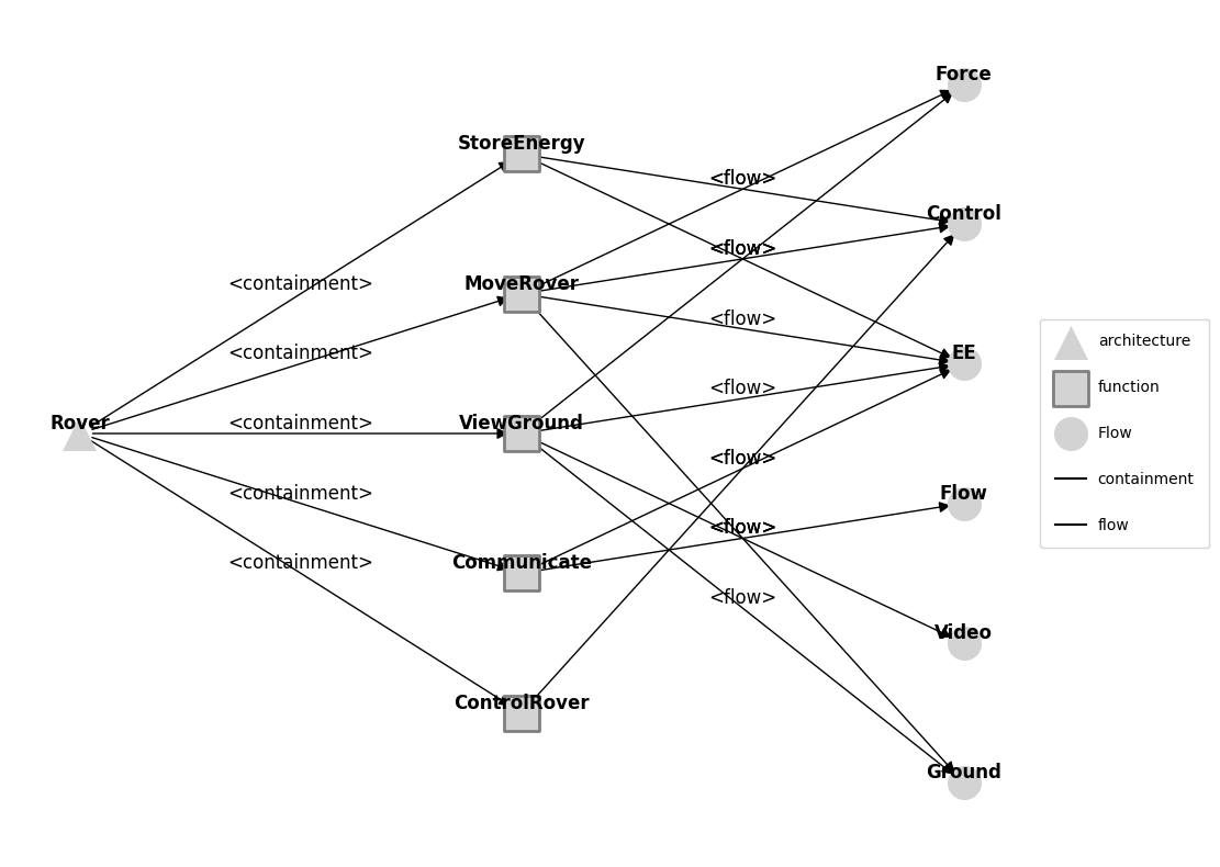
As shown, because the class for view ground and communicate are undefined, they are shown here as both instantiations of the Function class, which does not simulate. Additionally, Force, Ground, Video and Flow (used for comms) are left dangling since they aren’t actually connected to anything.
This same structure can also be visualized using the graphviz renderer, as shown below.
dot = mtg.draw_graphviz()
By default, draw uses matplotlib via networkx’s built-in plotting functions Other renderers are considered experimental and may not support every interface style argument without bugs.
However, graphviz is much more fully-featured and often creates nicer-looking plots. The reason it is not used by default (and why Graph was not build around it) is that graphviz needs to be installed externally.
Graph Views
While the FunctionArchitectureTypeGraph view shows the containtment relationships of the classes, the structural relationships between the model functions and flows can be viewed using the FunctionArchitectureFxnGraph, FunctionArchitectureFlowGraph and FunctionArchitectureGraph classes, shown below.
mfg = FunctionArchitectureFxnGraph(mdl)
fig, ax = mfg.draw()
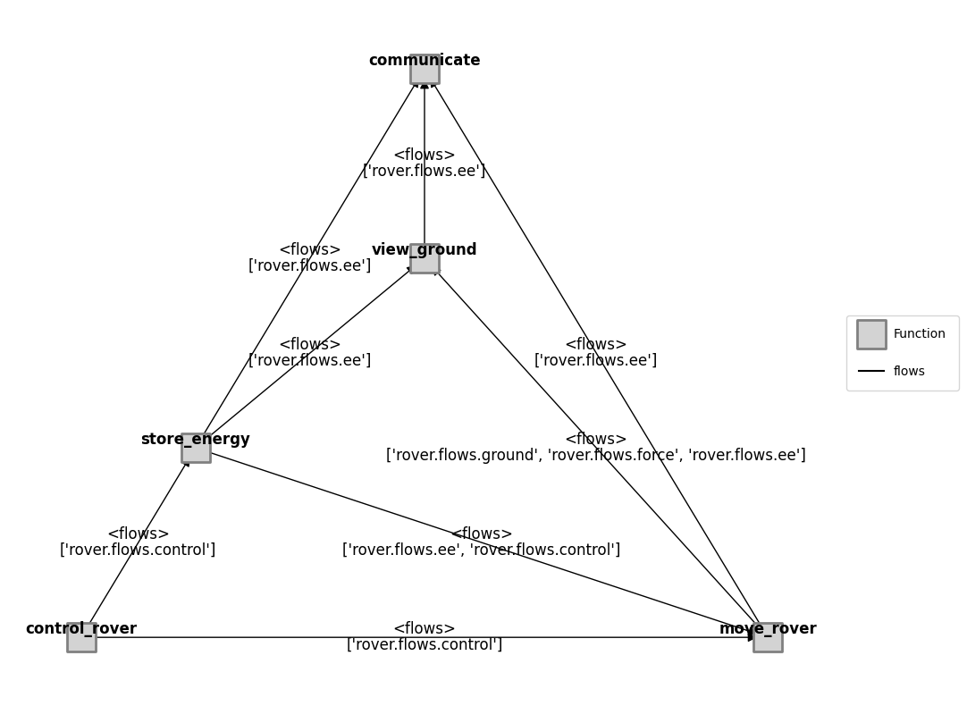
[i.get_label() for i in ax.get_legend().legend_handles]
['Function', 'flows']
mfg.edge_labels
Labels(title={('rover.fxns.control_rover', 'rover.fxns.move_rover'): '<flows>', ('rover.fxns.control_rover', 'rover.fxns.store_energy'): '<flows>', ('rover.fxns.store_energy', 'rover.fxns.communicate'): '<flows>', ('rover.fxns.store_energy', 'rover.fxns.view_ground'): '<flows>', ('rover.fxns.store_energy', 'rover.fxns.move_rover'): '<flows>', ('rover.fxns.move_rover', 'rover.fxns.communicate'): '<flows>', ('rover.fxns.move_rover', 'rover.fxns.view_ground'): '<flows>', ('rover.fxns.view_ground', 'rover.fxns.communicate'): '<flows>'}, title_style=EdgeLabelStyle(font_size=12, font_color='k', font_weight='normal', alpha=1.0, horizontalalignment='center', verticalalignment='bottom', clip_on=False, bbox={'alpha': 0}, rotate=False), subtext={('rover.fxns.control_rover', 'rover.fxns.move_rover'): "['rover.flows.control']", ('rover.fxns.control_rover', 'rover.fxns.store_energy'): "['rover.flows.control']", ('rover.fxns.store_energy', 'rover.fxns.communicate'): "['rover.flows.ee']", ('rover.fxns.store_energy', 'rover.fxns.view_ground'): "['rover.flows.ee']", ('rover.fxns.store_energy', 'rover.fxns.move_rover'): "['rover.flows.ee', 'rover.flows.control']", ('rover.fxns.move_rover', 'rover.fxns.communicate'): "['rover.flows.ee']", ('rover.fxns.move_rover', 'rover.fxns.view_ground'): "['rover.flows.ground', 'rover.flows.force', 'rover.flows.ee']", ('rover.fxns.view_ground', 'rover.fxns.communicate'): "['rover.flows.ee']"}, subtext_style=EdgeLabelStyle(font_size=12, font_color='k', font_weight='normal', alpha=1.0, horizontalalignment='center', verticalalignment='top', clip_on=False, bbox={'alpha': 0}, rotate=False))
Note the limitations with this representation. Specifically, flows mapped onto edges may duplicated each other (notice, for example, how many edges are listed with the ee flow! This
makes it difficult to visualize how multiple nodes are connected through the same flow
makes it difficult to label edges (since each edge may have a number of flows on it)
leads to many edge overlaps
The FunctionArchitectureFlowGraph is similarly limited:
mfg = FunctionArchitectureFlowGraph(mdl, check_info=False)
fig, ax = mfg.draw()
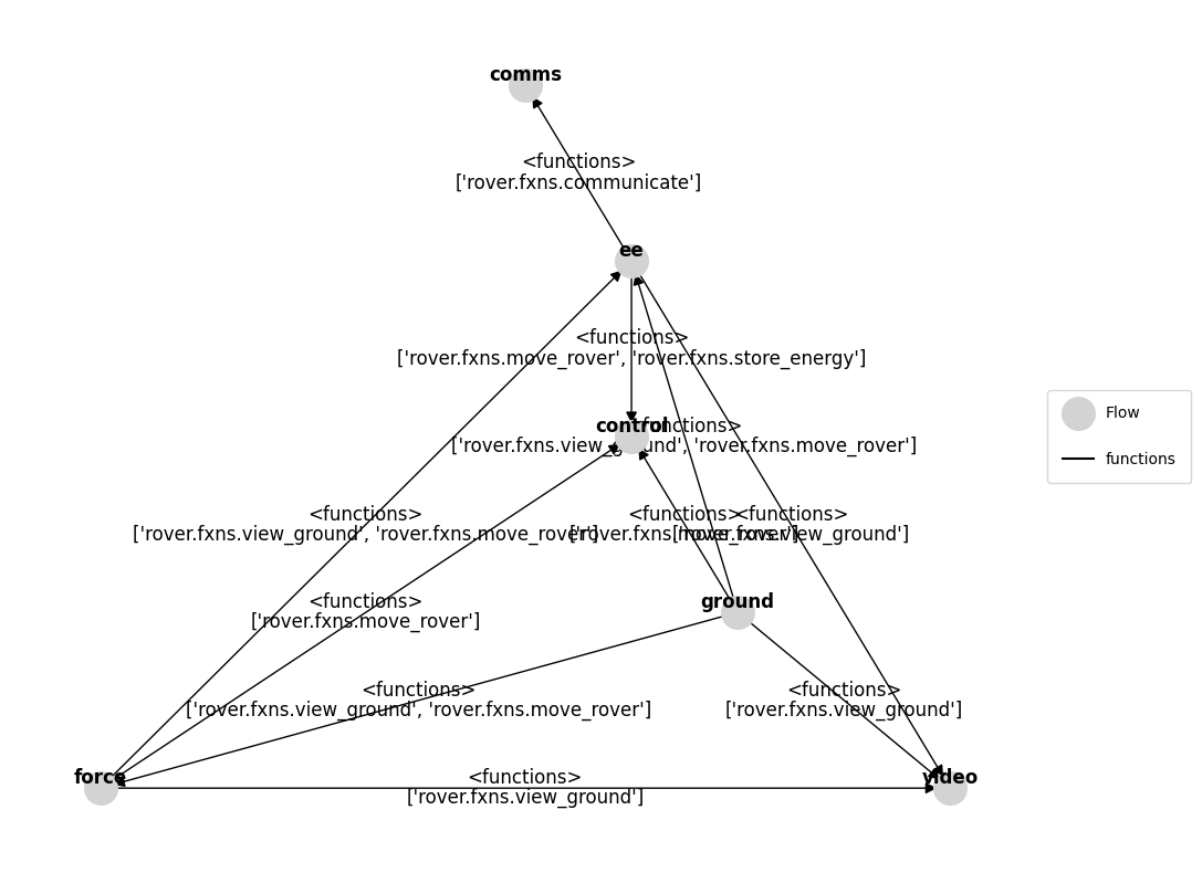
for n, v in mfg.g.nodes(data=True):
print(n)
rover.flows.ground
rover.flows.force
rover.flows.ee
rover.flows.video
rover.flows.control
rover.flows.comms
As a result, we usually use the standard FunctionArchitectureGraph class, which captures the full bipartite structure of models–where both functions and flows are nodes in the graph.
mg = FunctionArchitectureGraph(mdl)
mg.set_pos(**rover_pos)
fig, ax = mg.draw()
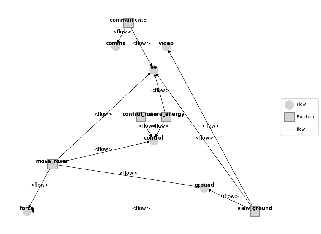
Note that these types are also compatible with graphviz. Graphviz output can be customized using options for the renderer (see http://www.graphviz.org/doc/info/attrs.html for all options)
For example:
dot = mg.draw_graphviz(layout='neato', overlap="voronoi")
Object Graphs
Object graphs can be used to view the containment and inheritance relationships of different objects.
from fmdtools.define.object.base import ObjectGraph
og = ObjectGraph(mdl)
d = og.draw_graphviz()
The default (shown above) is to show both inheritance and containment of the base object, without providing the structural characteristics. This can be changed using the options of ModelGraph:
og2 = ObjectGraph(mdl, with_inheritance = False)
d = og2.draw_graphviz()
og3 = ObjectGraph(mdl, with_containment = False)
d = og3.draw_graphviz()
A ModelGraph can also be generated for each Function, Flow (or other object) of the model, e.g.:
og4 = ObjectGraph(mdl.fxns['move_rover'])
d = og4.draw_graphviz()
This is a truncated representation of the underlying fmdtools class inheritance. For a full trace, the end_at_fmdtools option can be set to False:
og5 = ObjectGraph(mdl.fxns['move_rover'], end_at_fmdtools=False)
d = og5.draw_graphviz()
ObjectGraphs can also be used to view docs and code. Note that in this case the code must be defined in a separate file.
from examples.rover.rover_model import Rover as ExternalRoverModel
og6 = ObjectGraph(ExternalRoverModel().fxns['plan_path'], with_inheritance=False, get_source=True)
og6.set_node_labels(title='shortname', title2='classname', subtext='docs')
d = og6.draw_graphviz()
Full Model Containment Graph
By default, graph classes show a single level of containment hierarchy in order to remain tractable and represent the local definition of the given object/class.
We can view the entire containtment hierarchy of model objects using the recursive argument in any ModelGraph-type class:
from fmdtools.analyze.graph.model import ModelGraph
mg2 = ModelGraph(mdl, recursive=True)
d = mg2.draw_graphviz()
Run Order
To specify the run order of this model, the add_fxn method is used. The order of the call defines the run order of each instantiated function (Control_Rover -> Move_Rover -> Store_Energy -> View_Ground -> Communicate_Externally).
In addition to the functions which have been defined here, this model additionally has a number of functions which have not been defined (and will thus not execute). We can overlay these execution characteristics onto the graph using FunctionArchitectureGraph.set_exec_order.
help(FunctionArchitectureGraph.set_exec_order)
Help on function set_exec_order in module fmdtools.define.architecture.function:
set_exec_order(self, mdl, static={}, dynamic={}, next_edges={}, label_order=True, label_tstep=True)
Overlay FunctionArchitectureGraph execution order data on graph structure.
Parameters
----------
mdl : Model
Model to plot the execution order of.
static : dict/False, optional
kwargs to overwrite the default style for functions/flows in the static
execution step.
If False, static functions are not differentiated. The default is {}.
dynamic : dict/False, optional
kwargs to overwrite the default style for functions/flows in the dynamic
execution step.
If False, dynamic functions are not differentiated. The default is {}.
next_edges : dict
kwargs to overwrite the default style for edges indicating the flow order.
If False, these edges are not added. the default is {}.
label_order : bool, optional
Whether to label execution order (with a number on each node).
The default is True.
label_tstep : bool, optional
Whether to label each timestep (with a number in the subtitle).
The default is True.
mg.set_exec_order(mdl)
fig, ax = mg.draw()
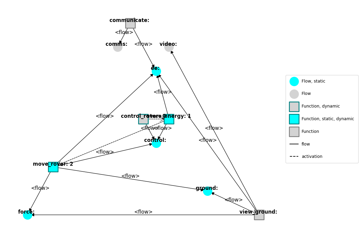
As shown, functions and flows active in the static propagation step are highlighted in cyan while the functions in the dynamic propagation step are shown (or given a border) in teal. Functions without behaviors are shown in light grey, and the run order of the dynamic propagation step is shown as numbers under the corresponding functions.
Additionally, by default the local timestep dt is labelled so we can see if/how it deviates from the overall model timestep–see, for example, the Store_Energy function.
In addition, Model.plot_dynamic_run_order can be used to visualize the dynamic propagation step.
mdl.plot_dynamic_run_order()
(<Figure size 640x480 with 1 Axes>, <Axes: >)
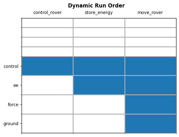
This plot shows that the dynamic execution step runs in the order defined in the Model module: first, Control_Rover, then, Store_Energy, and finally Move_Rover (reading left-to-right in the upper axis). The plot additionally shows which flows correspond to these function as it progresses through execution, which enables some understanding of which data structures are used or acted on at each execution time.
Behavior/Fault Visualization
To verify the static propagation of the short mode in the move_rover function, we can view the results of that scenario. As was set up, the intention of using the static propagation step was to enable the resulting fault behavior (a spike in current followed by a loss of charge) to occur in a single timestep.
In general, one can plot the effects of faults over time, using methods in plot, as shown below.
result, mdlhist = prop.one_fault(mdl, "move_rover", "short", 10, to_return='graph')
graph = result.faulty.tend.graph
graph
<fmdtools.define.architecture.function.FunctionArchitectureGraph at 0x2a1aa634d50>
fig, axs = mdlhist.plot_line(
'flows.ee.s.v',
'flows.ee.s.a',
'flows.control.s.power',
'flows.control.s.vel',
'fxns.store_energy.s.charge',
'fxns.store_energy.m.mode',
'fxns.move_rover.s.power', time_slice=10)

As shown, the static propagation step enables the mode to propagate back to the store_energy function (causing the no_charge fault) in the same timestep it is injected, even though it occurs later in the propagation order.
However, because the voltage and current output behaviors for the function are defined in the dynamic_behavior method of the store_energy function, these are only updated to their final value (of zero) at the next step. While this enables some visualization of the current spike, it may keep faults and behaviors from further propagating through the functions as desired. Thus, to enable this, one might reallocate some of the behaviors from the dynamic_behavior method to the static_behavior method.
Visualizing time-slices
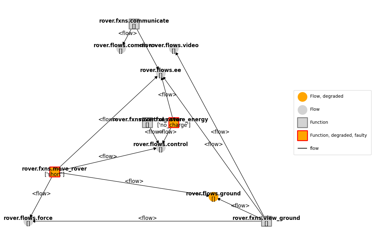
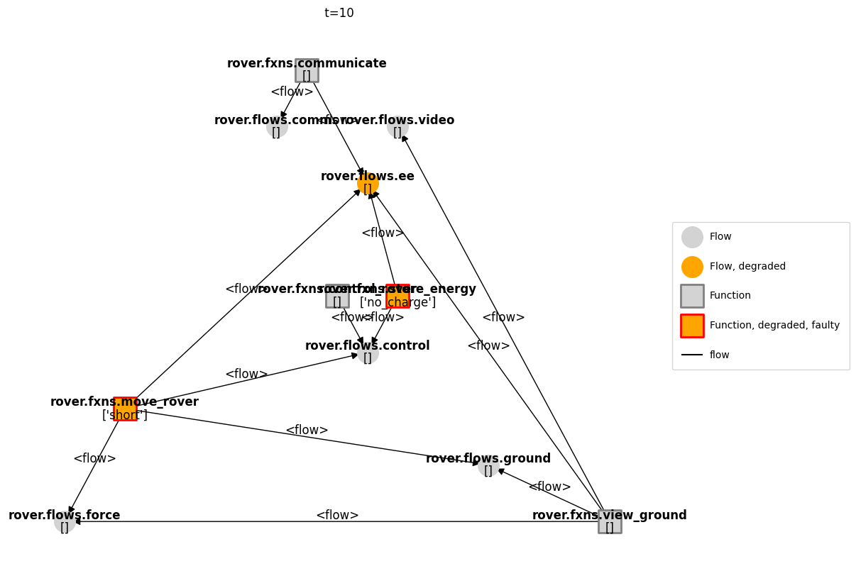
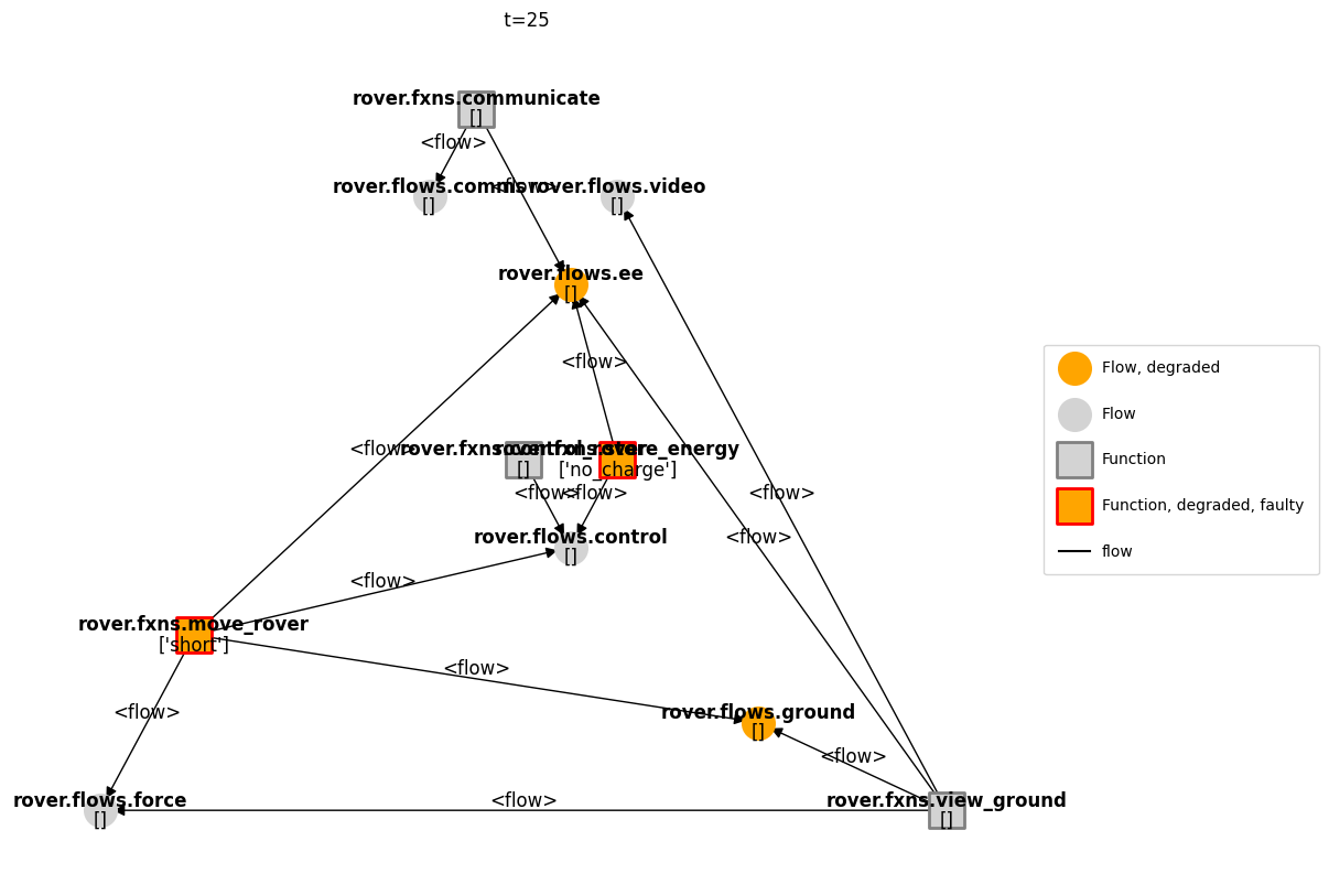
Contained in the result output in propagate.one_fault is the graph specified in to_return, which is a graph (multiple types may be provided). When output from propagate the Resgraph is by default given state information for each function/flow, as well as degraded and faulty properties which correlate with whether the State values deviate from those in the nominal.
Note that by default there are three main classifications for functions/flows visualized in this type of plot:
red: faulty function. Notes that the function is in a fault mode
orange: degraded function/flow. Nodes that the values of the flow or states of the function are different from the nominal scenario. Note that this is different than saying the values represent a problem, since contingency actions are also different between the nominal and faulty runs.
grey: nominal function/flow. This notes that there is nothing different between the nominal and faulty run in that function or flow.
These styles may be changed at will.
graph.set_pos(**rover_pos)
fig, ax = graph.draw()
dot = graph.draw_graphviz()
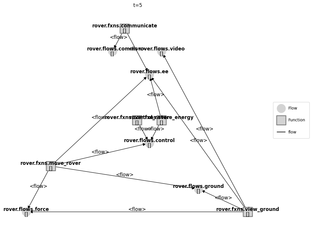
The resgraph only gives the state of the model at the final state. We might instead want to visualize the graph at different given times. This is performed with Graph.draw_from:
help(FunctionArchitectureGraph.draw_from)
Help on function draw_from in module fmdtools.define.architecture.base:
draw_from(self, *args, rem_ind=2, **kwargs)
Set from a history (removes prefixes so it works at top level).
rmg = FunctionArchitectureGraph(mdl)
rmg.set_pos(**rover_pos)
fig, ax = rmg.draw_from(5, mdlhist)
fig, ax = rmg.draw_from(10, mdlhist)
fig, ax = rmg.draw_from(25, mdlhist)
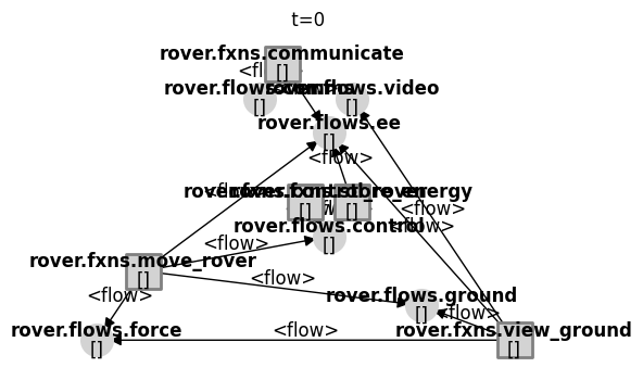
This can can be done automatically over a number of different times using Graph.animate:
help(FunctionArchitectureGraph.animate)
Help on function animate in module fmdtools.analyze.graph.model:
animate(self, history, times='all', figsize=(6, 4), **kwargs)
Successively animate a plot using Graph.draw_from.
Parameters
----------
history : History
History with faulty and nominal states
times : list, optional
List of times to animate over. The default is 'all'
figsize : tuple, optional
Size for the figure. The default is (6,4)
**kwargs : kwargs
Returns
-------
ani : matplotlib.animation.FuncAnimation
Animation object with the given frames
ani = rmg.animate(mdlhist)
from IPython.display import HTML
HTML(ani.to_jshtml())
Graph Metrics and Analysis
Beyond structural visualization, fmdtools provides methods to analyze graph properties and identify important nodes using centrality metrics.
Centrality Visualization
Centrality metrics help identify important nodes in the model structure. The plot_node_percentiles() method visualizes nodes colored by their importance according to different metrics.
import networkx as nx
# Create a fresh graph for centrality analysis
mg_cent = FunctionArchitectureGraph(mdl)
mg_cent.set_pos(**rover_pos)
# Visualize betweenness centrality (nodes that lie on paths between other nodes)
fig, ax = mg_cent.plot_node_percentiles(metric='betweenness', title='Betweenness Centrality')
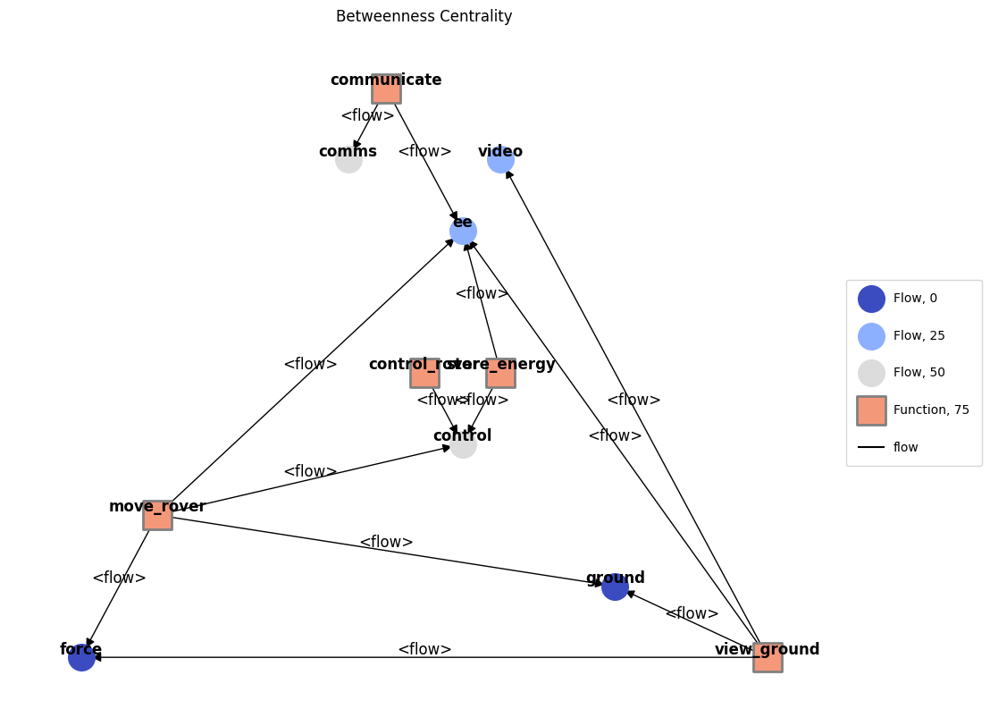
The plot shows nodes colored by quartile:
Light colors (low centrality): Nodes that are less central to information flow
Dark colors (high centrality): Nodes that bridge different parts of the system
Let’s try other centrality metrics:
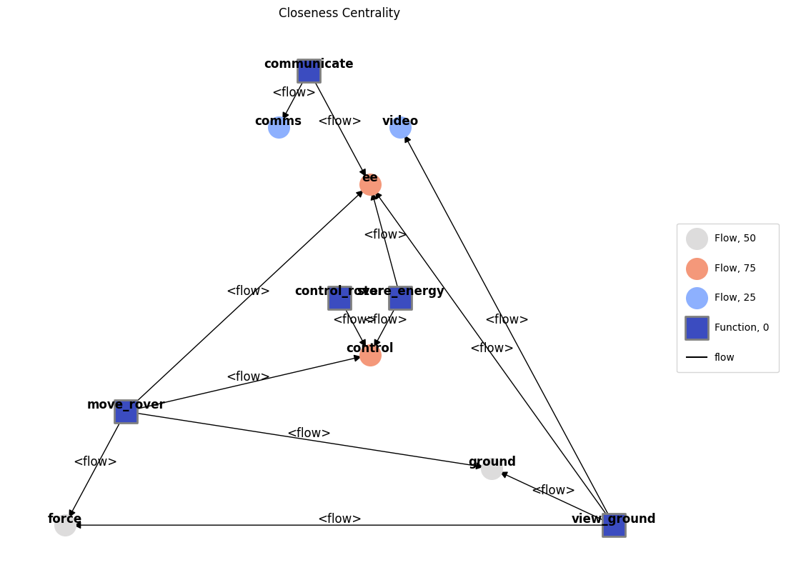
# Closeness centrality (nodes that are most central to the network)
mg_cent2 = FunctionArchitectureGraph(mdl)
mg_cent2.set_pos(**rover_pos)
fig, ax = mg_cent2.plot_node_percentiles(metric='closeness', title='Closeness Centrality')
# Degree centrality (nodes with most connections)
mg_cent3 = FunctionArchitectureGraph(mdl)
mg_cent3.set_pos(**rover_pos)
fig, ax = mg_cent3.plot_node_percentiles(metric='degree', title='Degree Centrality')

Custom Metrics
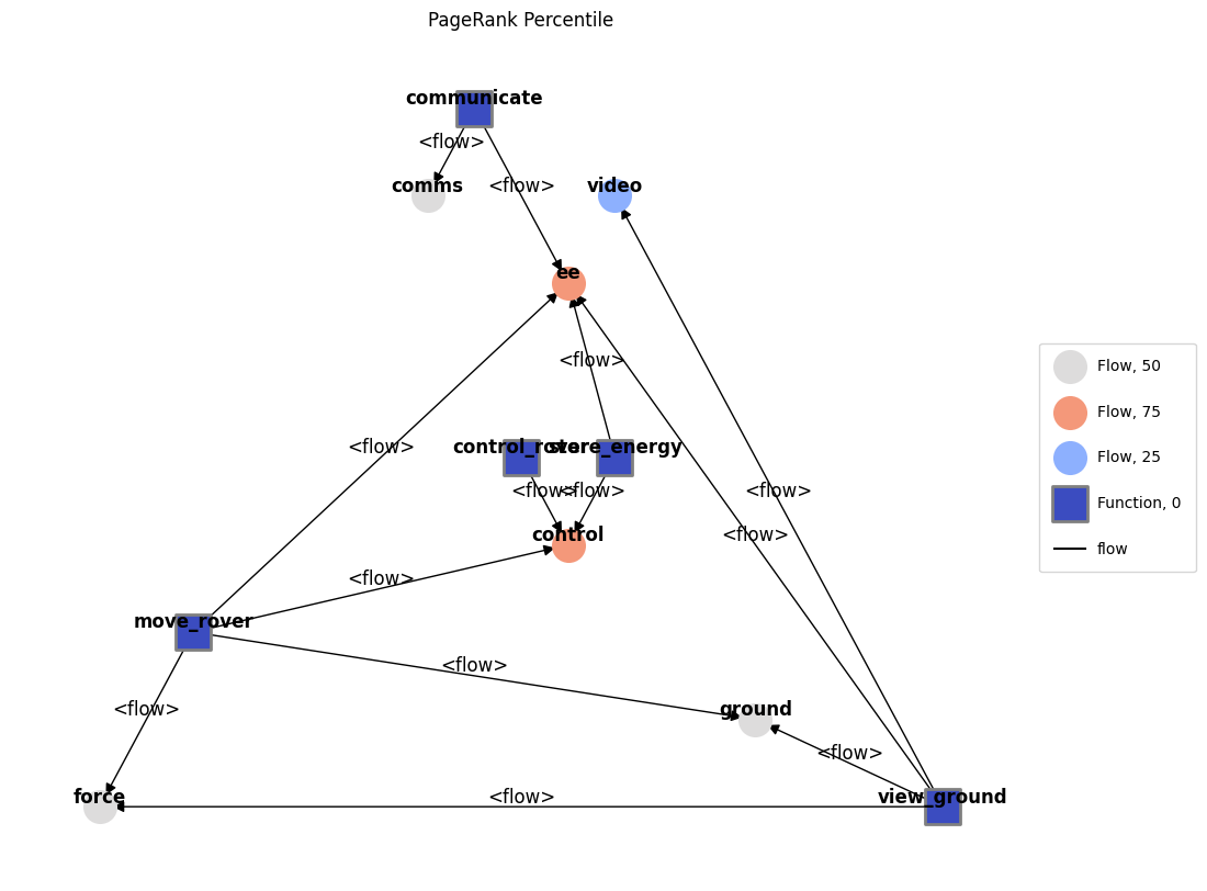
You can also use custom metric functions. For example, PageRank:
# Custom metric using PageRank
mg_cent4 = FunctionArchitectureGraph(mdl)
mg_cent4.set_pos(**rover_pos)
custom_metric = lambda g: nx.pagerank(g)
fig, ax = mg_cent4.plot_node_percentiles(metric=custom_metric, title='PageRank Percentile')
Graph Summary Statistics
The summary() method provides key metrics about the graph structure, useful for documentation and comparison:
mg_summary = FunctionArchitectureGraph(mdl)
summary = mg_summary.summary()
summary
{'num_nodes': 11,
'num_edges': 13,
'density': 0.11818181818181818,
'is_connected': True,
'num_components': 1,
'avg_degree': 2.3636363636363638,
'aspl': 2.4,
'modularity': 0.34319526627218944}
These metrics tell us:
Density: How connected the graph is (0 = no edges, 1 = fully connected)
Average Degree: Average number of connections per node
Average Shortest Path Length (ASPL): Average distance between nodes (only for connected graphs)
Modularity: Strength of division into communities (higher = more modular)
Comparing Model Variants
The compare_with() method helps compare different model architectures. This is useful for:
Comparing design alternatives
Tracking model evolution across versions
Analyzing the impact of architectural changes
Let’s compare the Rover model with the Pump model:
from examples.pump.ex_pump import Pump
# Create graphs for both models
rover_graph = FunctionArchitectureGraph(Rover())
pump_graph = FunctionArchitectureGraph(Pump())
# Compare the two models
comparison = rover_graph.compare_with(pump_graph)
comparison
{'nodes_added': {'pump.flows.ee_1',
'pump.flows.sig_1',
'pump.flows.wat_1',
'pump.flows.wat_2',
'pump.fxns.export_water',
'pump.fxns.import_ee',
'pump.fxns.import_signal',
'pump.fxns.import_water',
'pump.fxns.move_water'},
'nodes_removed': {'rover.flows.comms',
'rover.flows.control',
'rover.flows.ee',
'rover.flows.force',
'rover.flows.ground',
'rover.flows.video',
'rover.fxns.communicate',
'rover.fxns.control_rover',
'rover.fxns.move_rover',
'rover.fxns.store_energy',
'rover.fxns.view_ground'},
'edges_added': {('pump.fxns.export_water', 'pump.flows.wat_2'),
('pump.fxns.import_ee', 'pump.flows.ee_1'),
('pump.fxns.import_signal', 'pump.flows.sig_1'),
('pump.fxns.import_water', 'pump.flows.wat_1'),
('pump.fxns.move_water', 'pump.flows.ee_1'),
('pump.fxns.move_water', 'pump.flows.sig_1'),
('pump.fxns.move_water', 'pump.flows.wat_1'),
('pump.fxns.move_water', 'pump.flows.wat_2')},
'edges_removed': {('rover.fxns.communicate', 'rover.flows.comms'),
('rover.fxns.communicate', 'rover.flows.ee'),
('rover.fxns.control_rover', 'rover.flows.control'),
('rover.fxns.move_rover', 'rover.flows.control'),
('rover.fxns.move_rover', 'rover.flows.ee'),
('rover.fxns.move_rover', 'rover.flows.force'),
('rover.fxns.move_rover', 'rover.flows.ground'),
('rover.fxns.store_energy', 'rover.flows.control'),
('rover.fxns.store_energy', 'rover.flows.ee'),
('rover.fxns.view_ground', 'rover.flows.ee'),
('rover.fxns.view_ground', 'rover.flows.force'),
('rover.fxns.view_ground', 'rover.flows.ground'),
('rover.fxns.view_ground', 'rover.flows.video')},
'structure_similarity': 0.0,
'summary_this': {'num_nodes': 11,
'num_edges': 13,
'density': 0.11818181818181818,
'is_connected': True,
'num_components': 1,
'avg_degree': 2.3636363636363638,
'aspl': 2.4,
'modularity': 0.34319526627218944},
'summary_other': {'num_nodes': 9,
'num_edges': 8,
'density': 0.1111111111111111,
'is_connected': True,
'num_components': 1,
'avg_degree': 1.7777777777777777,
'aspl': 2.4444444444444446,
'modularity': 0.375}}
print("\nRover Summary:")
for key, value in comparison['summary_this'].items():
print(f" {key}: {value}")
print("\nPump Summary:")
for key, value in comparison['summary_other'].items():
print(f" {key}: {value}")
Rover Summary:
num_nodes: 11
num_edges: 13
density: 0.11818181818181818
is_connected: True
num_components: 1
avg_degree: 2.3636363636363638
aspl: 2.4
modularity: 0.34319526627218944
Pump Summary:
num_nodes: 9
num_edges: 8
density: 0.1111111111111111
is_connected: True
num_components: 1
avg_degree: 1.7777777777777777
aspl: 2.4444444444444446
modularity: 0.375
The Graph class has many more capabilities for performing graph visualization and analysis on model structures of interest, leveraging the powerful networkx library. See the Graph documentation for more.