Rover Response Optimization
This notebook shows how variables in an fmdtools model can be optimized for resilience.
from fmdtools.sim.sample import SampleApproach, FaultSample, FaultDomain, ParameterDomain
import fmdtools.analyze as an
import fmdtools.sim.propagate as prop
from fmdtools.sim.search import ParameterSimProblem
import matplotlib.pyplot as plt
import multiprocessing as mp
import time
Model is in defined rover_model.py
from examples.rover.rover_model import Rover, RoverParam
Optimization
Here we define the optimization problem for the rover.
We use a parallel pool, staged execution, and minimal tracking options to lower computational cost as much as possible.
mdl = Rover(sp={'end_condition': ''}, track={'flows':{"ground":"all", "pos": "all"}})
#rover_prob = search.ProblemInterface("rover_problem", mdl, pool=mp.Pool(5), staged=True, track=track)
mdl.h
flows.ground.r.probdens:      array(151)
flows.ground.s.in_bound:      array(151)
flows.ground.c.r.probdens:    array(151)
flows.ground.ga.points.start: array(151)
flows.ground.ga.points.end:   array(151)
flows.ground.ga.lines.line:   array(151)
flows.pos.s.x:                array(151)
flows.pos.s.y:                array(151)
flows.pos.s.vel:              array(151)
flows.pos.s.ux:               array(151)
flows.pos.s.uy:               array(151)
mdl.p
RoverParam(ground=GroundParam(linetype='sine', amp=1.0, period=6.283185307179586, radius=20.0, x_start=10.0, y_end=10.0, x_min=0.0, x_max=30.0, x_res=0.1, path_buffer_on=0.2, path_buffer_poor=0.3, path_buffer_near=0.4, dest_buffer_on=1.0, dest_buffer_near=2.0), correction=ResCorrection(ub_f=10.0, lb_f=-1.0, ub_t=10.0, lb_t=0.0, ub_d=2.0, lb_d=-2.0, cor_d=0.0, cor_t=0.0, cor_f=0.0), degradation=DegParam(friction=0.0, drift=0.0), drive_modes={'mode_options': 'set'})
Here we will be optimizing over faults in the drive system at 3 points during the drive simulation interval:
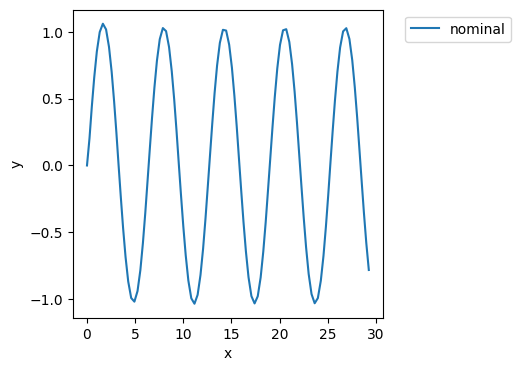
endresults, mdlhist = prop.nominal(Rover())
phasemap = an.phases.from_hist(mdlhist)
fault_domain = FaultDomain(mdl)
fault_domain.add_all_fxnclass_modes('Drive')
fault_sample = FaultSample(fault_domain, phasemap['plan_path'])
fault_sample.add_fault_phases('drive',  args=(3,))
fig, ax = mdlhist.plot_trajectories("flows.pos.s.x", "flows.pos.s.y")
The variables are the correction factors int the fault management:
pd = ParameterDomain(RoverParam)
pd.add_variables("correction.cor_f", "correction.cor_d", "correction.cor_t", lims={"correction.cor_f":(0, 1),
                                                                                         "correction.cor_d":(-1, 1),
                                                                                         "correction.cor_t":(-1, 1)})
pd
ParameterDomain with:
 - variables: {'correction.cor_f': (0, 1), 'correction.cor_d': (-1, 1), 'correction.cor_t': (-1, 1)}
 - constants: {}
 - parameter_initializer: RoverParam
Now we setup the optimization problem using ParameterSimProblem
We can define multiple objectives, below we will use the end distance and total_deviation from classify.
class RoverProb(ParameterSimProblem):
    def init_problem(self, **kwargs):
        self.add_parameterdomain(pd)
        self.add_sim(mdl, "fault_sample", fault_sample, **kwargs)
        self.add_result_objective('f1', 'endclass.end_dist')
        self.add_result_objective('f2', 'endclass.tot_deviation')
rover_prob = RoverProb()
rover_prob
RoverProb with:
VARIABLES
 -correction.cor_f                                              nan
 -correction.cor_d                                              nan
 -correction.cor_t                                              nan
OBJECTIVES
 -f1                                                            nan
 -f2                                                            nan
Here we do some basic timing:
rover_prob.f1(0.5,0.5,0.5)
a=time.time()
rover_prob.f1(0.6,0.5,0.5)
t=time.time()-a
t
10.915723085403442
rover_prob
RoverProb with:
VARIABLES
 -correction.cor_f                                           0.6000
 -correction.cor_d                                           0.5000
 -correction.cor_t                                           0.5000
OBJECTIVES
 -f1                                                      1201.3735
 -f2                                                        17.4880
Alternatively, we can use:
rover_prob.time_execution(0.7,0.5,0.5)
10.422291278839111
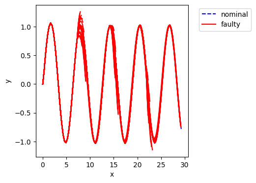
fig, ax = rover_prob.hist.plot_trajectories("flows.pos.s.x", "flows.pos.s.y")
rover_prob
RoverProb with:
VARIABLES
 -correction.cor_f                                           0.7000
 -correction.cor_d                                           0.5000
 -correction.cor_t                                           0.5000
OBJECTIVES
 -f1                                                      1206.7123
 -f2                                                        17.4456
Rover Optimization:
from pymoo.optimize import minimize
from pymoo.algorithms.soo.nonconvex.pattern import PatternSearch
from pymoo.problems.functional import FunctionalProblem
import numpy as np
Covert optimization problem into a pymoo problem
from multiprocessing import Pool
rover_prob = RoverProb(pool=Pool(4), close_pool=False)

n_var = len(rover_prob.variables)
x_low = np.array([])
x_up = np.array([])
for bound in rover_prob.parameterdomain.variables.values():
    x_low = np.append(x_low, bound[0])
    x_up = np.append(x_up, bound[1])

obj = [lambda x: rover_prob.f1(*x)]
pymoo_prob = FunctionalProblem(n_var, obj, xl = x_low, xu= x_up)
arg={}
pymoo_prob._evaluate([0.7,0.5,0.5],arg)
arg
{'F': array([1206.7123064]),
 'G': array([], dtype=float64),
 'H': array([], dtype=float64)}
Run optimizaion algorithm..
algorithm=PatternSearch(x0=np.array([0.7,0.5,0.5]))
from pymoo.termination import get_termination
# early termination
termination = get_termination("n_eval", 13)
res = minimize(pymoo_prob, algorithm, termination=termination, verbose=True)
=================================================
n_gen  |  n_eval  |     f_avg     |     f_min
=================================================
     1 |        1 |  1.206712E+03 |  1.206712E+03
     2 |        6 |  1.203385E+03 |  1.200057E+03
     3 |       13 |  1.200057E+03 |  1.200057E+03
res.X
array([0.575, 0.5 , 0.75 ])
opt_x = [ 0.16970361, -0.78522209, 0.10777078]
Results visualization
Here we look at the optimized results and compare with the starting results:
rover_prob.f1(0.16970361, -0.78522209, 0.10777078)
1192.4808142724964
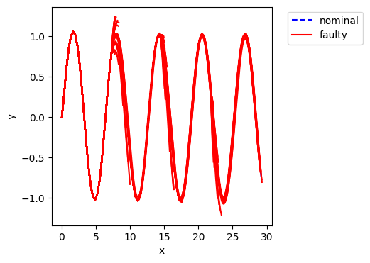
fig, ax = rover_prob.hist.plot_trajectories("flows.pos.s.x", "flows.pos.s.y")
rover_prob
RoverProb with:
VARIABLES
 -correction.cor_f                                           0.1697
 -correction.cor_d                                          -0.7852
 -correction.cor_t                                           0.1078
OBJECTIVES
 -f1                                                      1192.4808
 -f2                                                        17.9378
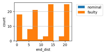
fig, ax = rover_prob.res.plot_metric_dist('end_dist')
starting solution:
rover_prob.f1(0.7,0.5,0.5)
1206.7123064010684
fig, ax = rover_prob.hist.plot_trajectories("flows.pos.s.x", "flows.pos.s.y")
rover_prob
RoverProb with:
VARIABLES
 -correction.cor_f                                           0.7000
 -correction.cor_d                                           0.5000
 -correction.cor_t                                           0.5000
OBJECTIVES
 -f1                                                      1206.7123
 -f2                                                        17.4456
fig, ax = rover_prob.res.plot_metric_dist('end_dist')
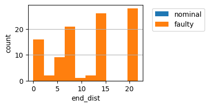
As shown, while the optimized correction factors don’t mitigate all scenarios, they do increase the number of scenarios that are mitigated.
rover_prob.close_pool()