Intro to fmdtools
Overview {.smaller}
Overview of fmdtools
Purpose
Project Structure
Common Classes/Functions
Basic Syntax
Coding Activity - Pump or Drone Example
In the
examples/water_pumporexamples/multirotor_dronefoldersModel
Workbook:
Model Instantiation
Simulation
Visualization/Analysis
Prerequisites
Ideally, some pre-existing Python and Git knowledge
Python distribution (anaconda or uv)
Ideally this is already set up!
Download/install from:
https://www.anaconda.com/products/individual
https://github.com/astral-sh/uv
A git interface
Github Desktop (graphical git environment)
git-scm (stand-alone CLI)
Motivation: Modeling System Resilience
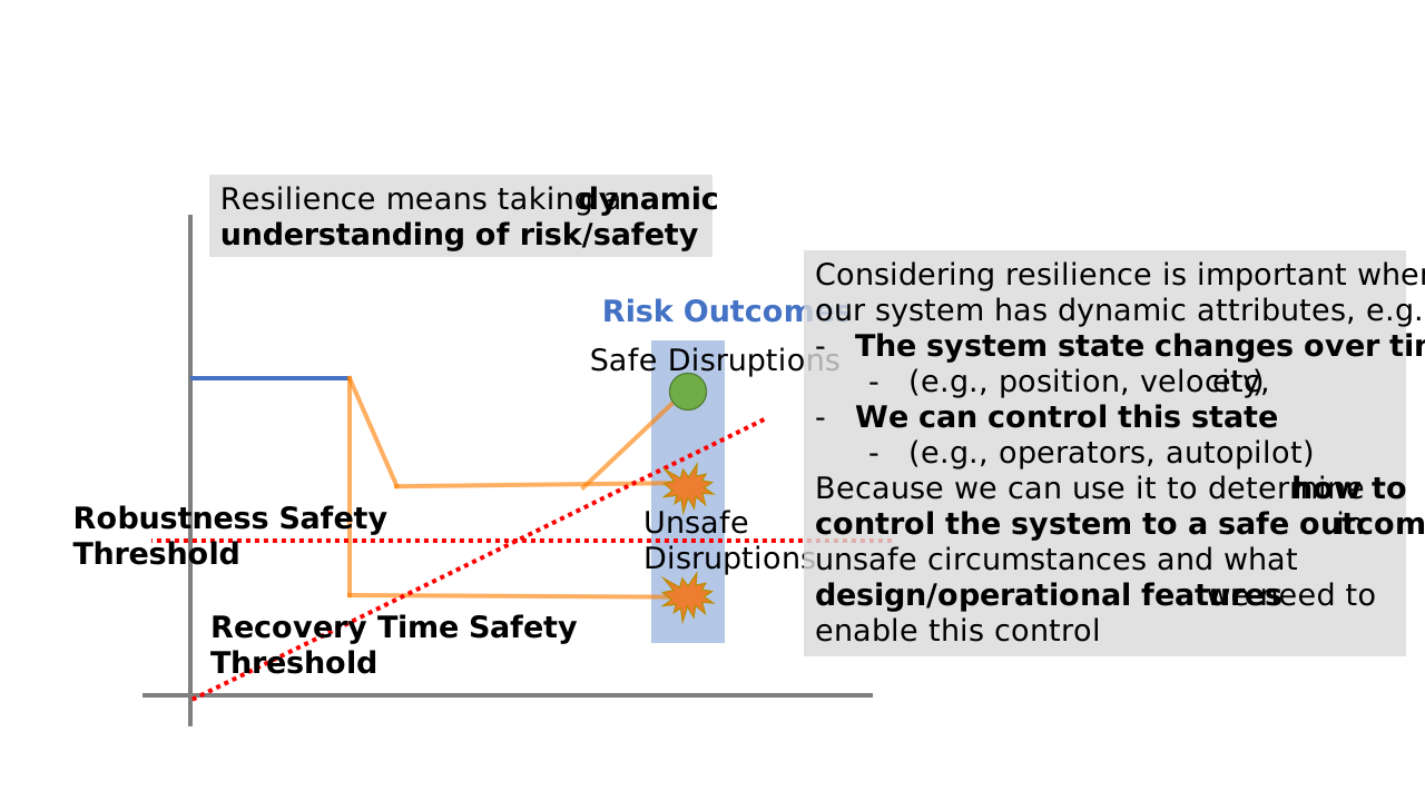
Resilience means taking a dynamic understanding of risk and safety
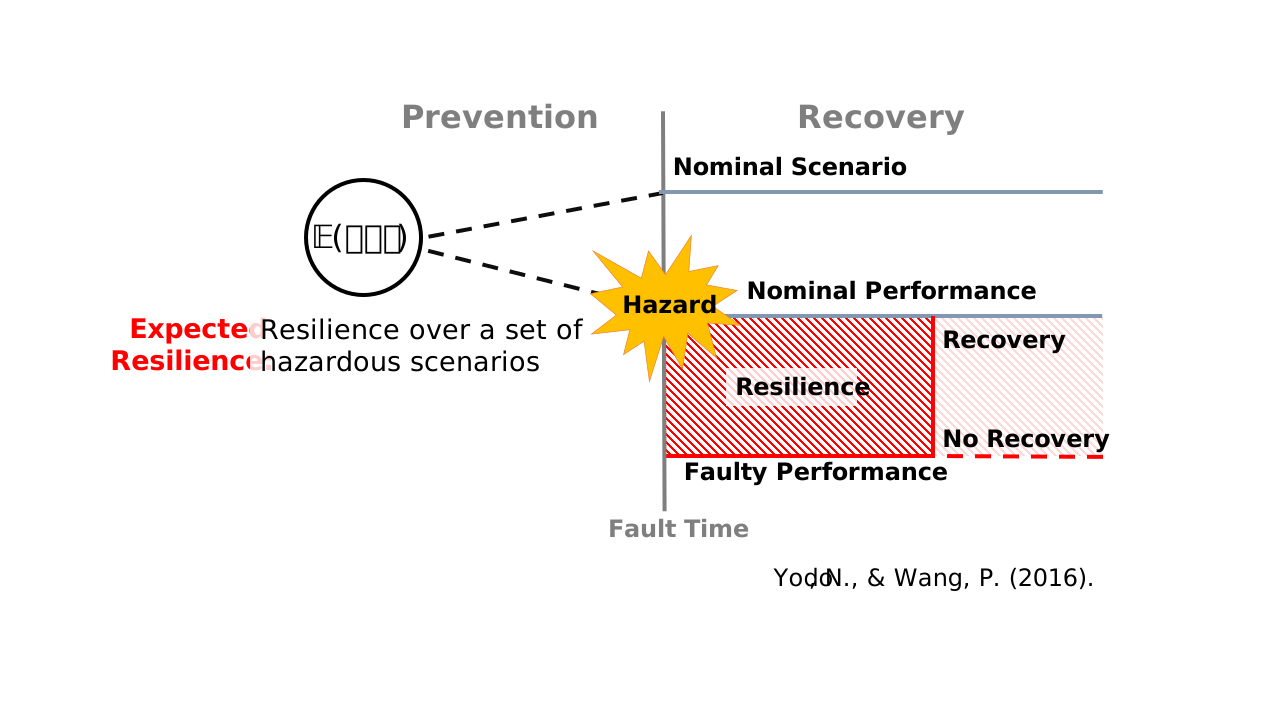
Why is Resilience Important?
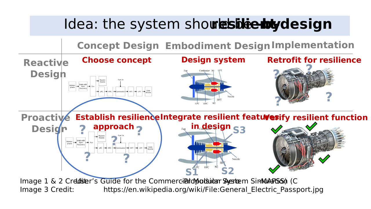
Enabling a proactive design process - especially when we don’t have data
Why fmdtools? Possible Competitors:
Uncertainty Quantification tools: (e.g. OpenCossan)
Does not incorporate fault modeling/propagation/visualization aspects
MATLAB/modelica/etc. Fault Simulation tools
Rely on pre-existing model/software stack–Useful, but often difficult to hack/extend (not open-source)
Safety Assessment tools: (e.g. Alyrica, Hip-Hops)
Focused on quantifying safety, not necessarily resilience
As a result, use different model formalisms!
Why fmdtools? Pros: {.smaller}
Highly Expressive, modular model representation.
faults from any component can propagate to any other connected component
highly-extensible code-based behavior representation
modularity enables complex models and modelling use-cases
Research-oriented:
Written in/relies on the Python stack
Open source/free software
Enables design:
Models can be parameterized and optimized!
Plug-and-play analyses and visualizations
Why not fmdtools? Cons:
You already have a pre-existing system model
fmdtools models are built in fmdtools
if you have a simulink/modelica model, you may just want to use built-in tools
You want to use this in production
fmdtools is Class E Software and thus mainly suitable for research (or, at least, we don’t guarantee it)
Somewhat dynamic development history
What is fmdtools? A Python package for design, simulation, and analysis of resilience.
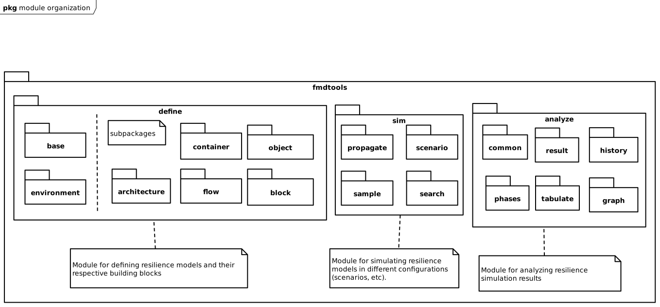
What is fmdtools? Repo Structure
/src/fmdtools: installable package directory/examples: example models with demonstrative notebooks and tests/docs: HTML Documentation (source files at/docs-source)/tests: stand-alone tests (and testing rigs)Basic information:
README.md,CONTRIBUTORS.md,PUBLICATIONS.md,LICENSE,fmdtools_Individual_CLA.pdf, etc.Config/test files:
requirements.txt,pyproject.toml,index.rst, etc.
Activity: Download and Install fmdtools {.smaller}
repo link: https://github.com/nasa/fmdtools/
set up repo:
create
path/to/fmdtoolsfolder for repo(usually in
/documents/GitHub)
clone git into folder:
git clone https://github.com/nasa/fmdtools.gitcan also use webpage
package installation:
anaconda: Open Python from anaconda (e.g., open Spyder) and install with
pip install -e /path/to/fmdtoolsuv: run
uv pip install .from fmdtools repository
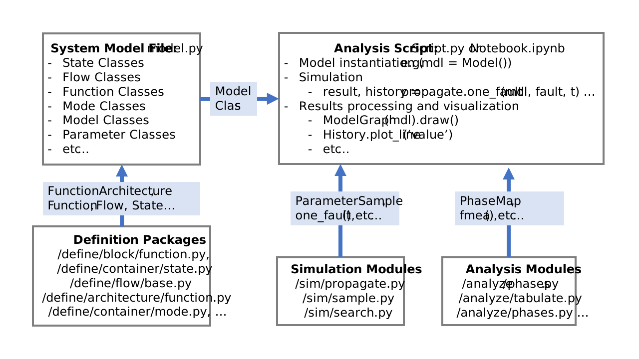
Analysis Workflow/Structure
Defining a Model {.smaller}
What do we want out of a model?
What behaviors and how much fidelity do we need?
What functions/components and interactions make up the system?
One function or multiple functions?
Is it a controlled system? Are there multiple agents?
What type of simulation do we want to run?
Single-timestep vs multi-timestep vs network
What scenarios do we want to study and how?
Failure modes and faulty behaviors
Disturbances and changes in parameters
What are the possible effects of hazards and how bad are they?
By what metrics?
Defining a Model
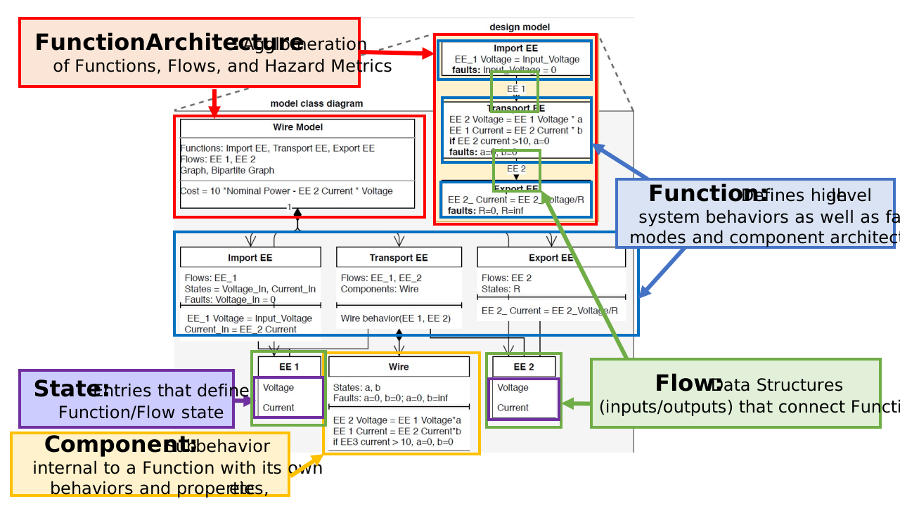
Concept: Static Propagation

In a single timestep, functions with static_behavior() methods simulate until behaviors converge (i.e., no new state values)
Concept: Propagation over Time {.smaller}
::::: columns
::: {.column width=”50%”}
 :::
:::
::: {.column width=”50%”}
Model increments (simulated + history updated) over each time-step until a defined final time-step or specified indicator returns true.
Functions with
dynamic_behavior()run once in defined order ::: :::::
Python Concept: Classes and Object-Oriented Programming {.smaller}
Classes are the core of object-oriented programming. A class in python might look like:
class Hello(object):
    a = 3 # <- Class variables define data used by all objects
    def __init__(self, x=1, y=2): #<- This is a "dunder" method to instantiate the class
        self.x = x
        self.y = y

    def sum(self):
        return self.x + self.y + self.a
Classes are instantiated to form objects, which we can then use to manipulate data, e.g.:
>>> hi = Hello(x=2, y=2)
>>> hi.sum()
7
Why classes and objects? {.smaller}
Classes give you the ability to group data and methods together to satisfy an overall use-case
Classes define the “template”–what should an object include, be able to do, how should it be instantiated, etc.
Inheritance–you can create subclasses that creating new variants for a given system with specific properties (e.g., Ferrari might be a subclass of a Car class)
Principle of encapsulation: Object-oriented programming give you control of what the user (or environment sees) versus what should be “internal”
Organization: You always know what methods are supposed to act on what data
Independence: New objects are independent of old objects, so, e.g., if you want a new sim while keeping the old one you can do that
Python dataclasses (and similar) {.smaller}
The fmdtools library extends the recordclass package to define dataclasses: https://github.com/intellimath/recordclass
from recordclass import dataobject
class Point(dataobject):
    x: int = 1 # <- Field for variable x
    y: int = 2 # <- Field for variable y
Dataclasses let one define the data as fields and then lets you directly instantiate the class based on the data, e.g.:
>>> p = Point(2, 3)
>>> p.x
2
Dataclasses are used in the fmdtools library for its Container classes which you as a developer then use!
Containers - The building blocks of simulations {.smaller}
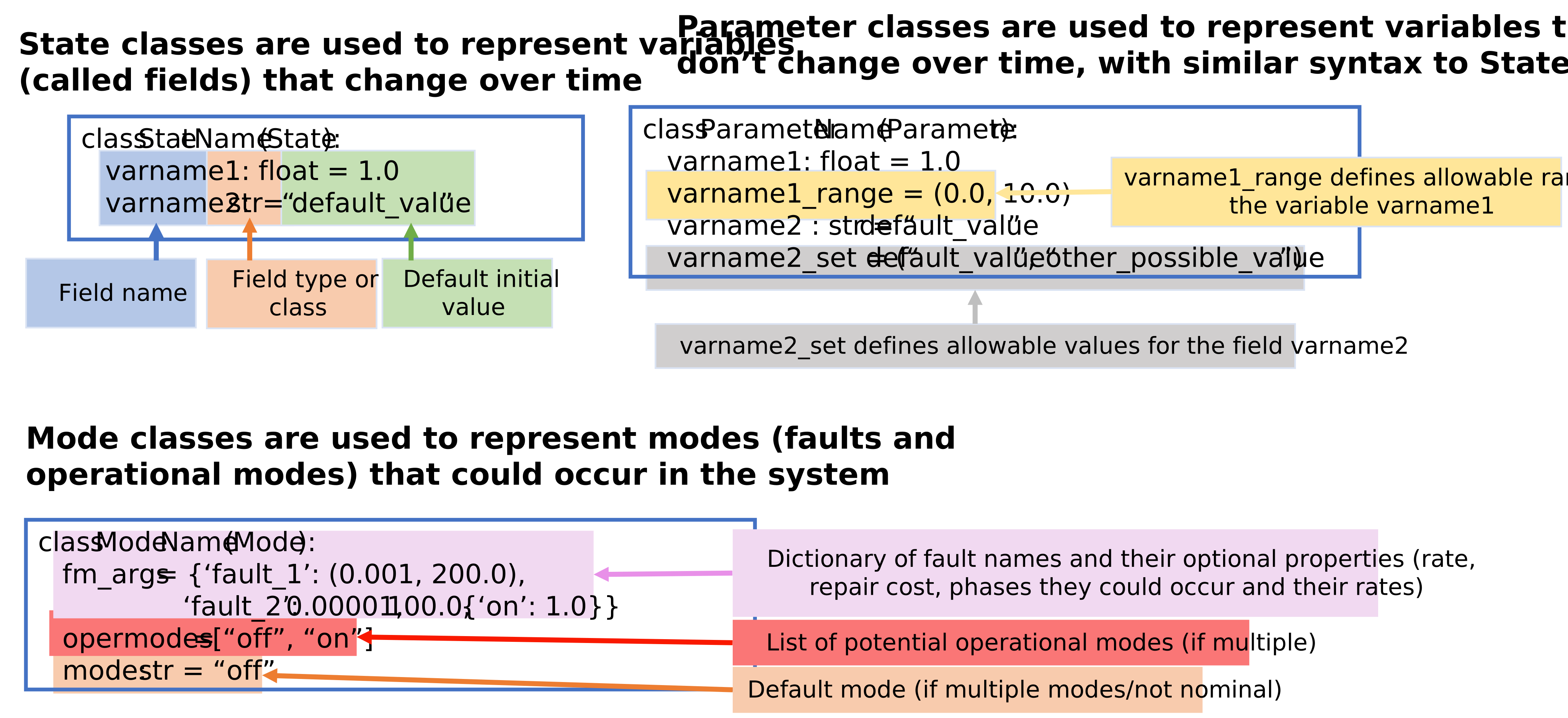 - Containers are used to define various attributes of Functions and Flows
Click for full code template
class StateName(State): # defining state class
    varname1: float = 1.0 # defining a float variable that defaults to 1.0
    varname2: str = “default_value” # defining a string variable that defaults to "default_value"

class ParameterName(Parameter): # defining parameter class
    varname1: float = 1.0 # defining a float varname1 that defaults to 1.0
    varname1_range = (0.0, 10.0) # defining an allowable range for varname1 (optional to bound model validity)
    varname2 : str = “default_value”
    varname2_set = (“default_value”, “other_possible_value”) # defining a set of allowable values for varname2

class ModeName(Mode): # defining mode class
    fault_faultname1 = (0.001, 200.0) # defining the fault mode faultname1 and its rate and cost
    fault_faultname2 = (0.00001, 100.0, {‘on’: 1.0}) # defining the fault mode faultname2 and its rate, cost, and applicable phases of operation (all in the "on" operational mode)
    opermodes = (“off”, "on") # defining the allowable operational modes ("off" and "on")
    mode: str = "off" # Declaring a default or initial mode. Otherwise the mode will be "nominal" unless there is a fault.
Class aggregation in fmdtools BaseObject {.smaller}
In fmdtools, BaseObject classes (Functions, Flows, etc.) aggregate Containers classes, allowing you to instantiate multiple at the same time, e.g., in the class:
class ExampleObject(BaseObject):
    container_s = StateName
container_sattaches theStateNameclass to the ExampleObject class as a containerOur object class instantiates it to the variable
s, e.g.:
>>> ex = ExampleObject()
>>> ex.s.varname1
1.0
Main classes in fmdtools {.smaller}

Containers are used to represent properties of Objects (all classes below)
Blocks are the main behaviors of the system (e.g., Functions or Components)
Flows connect functions (and are thus a part of their definition)
Architectures are used to instantiate and connect Blocks with Flows
Flow Code Template
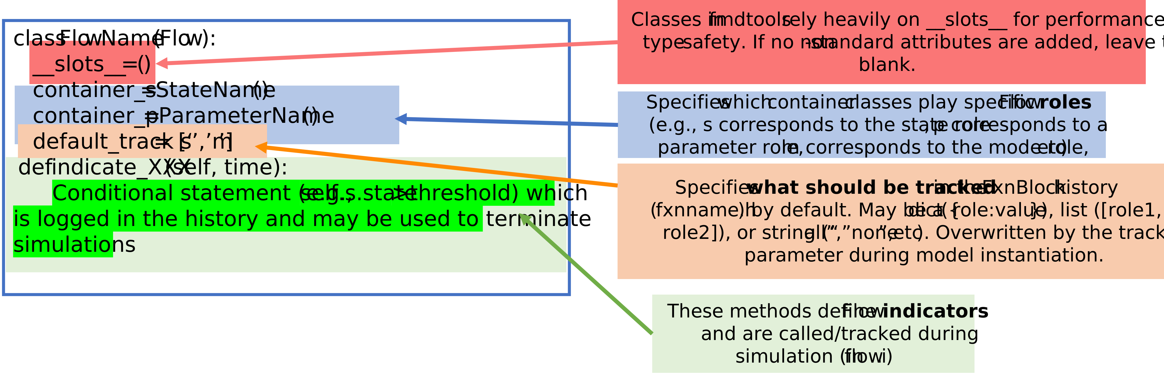
Flows represent connections or shared variables between different functions. Think of them as Function inputs/outputs.
Flows are build from container classes like states, along with their own methods/variables.
Click for full code template
class FlowName(Flow): # defining flow class
    container_s = StateName # Will initialize the state StateName at self.s
    container_p = ParameterName # Will initialize the parameter ParameterName at self.p
    default_track = ['s’, 'i'] # Optional arguments to define that the state "s" and indicators "i" will be tracked (otherwise everything will be tracked)

def indicate_varname_too_high(self): # Optional conditional using `indicate_XX` syntax
    return self.s.varname1 > 1.0 # if the variable varname1 is greater than one, the indicator will return True
Function Code Template
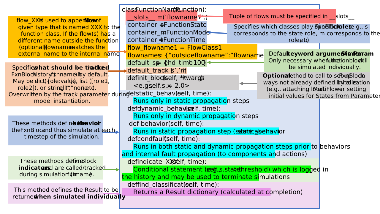
Click for full code template
class FunctionName(Function):
    container_s = StateName # Will initialize the state StateName at self.s
    container_m = ModeName  # Will initialize the mode ModeName at self.m
    container_t = FunctionTime  # Will initialize the time container FunctionTime at self.t
    flow_connection = FlowName # Will initialize or attach the flow FlowName at self.connection.
    flownames = {'outsideflowname': 'connection'} # Optionally redefines a flow with an external name with a local internal name
    default_sp = {'end_time': 100} # Defines and end time if simulating this function individually
    default_track = ['s','m'] # Optionally defines which attributes to track (the state and mode)

def init_block(self, **kwargs): # Optional method for initializing variables values. May be helpful local instantiation when using MultiFlow and CommsFlow classes.
    self.s.varname1 = 2.0 # This would be useful if there were multiple usages to the StateName class and this one needed to be 2.0 at the start of the sim

def static_behavior(self): # Defines top-level behavior to be simulated during a timestep until behavior converges (useful for propagation)
    if self.m.has_fault("faultname"): # Often used for failure logic
        self.s.varname1 = 10.0 # Best practice is to change variables to a set value. Do not increment values in static_behavior or behavior will not converge.
    self.connection.s.varname1 = self.s.varname1 # Always access/modify flows from their defined names on instantiation, not their class variables.


def dynamic_behavior(self): # Defines top-level behavior to be simulated once during a timestep.
    self.s.varname2 += self.connection.s.varname1 # Useful for incrementing behavior over time.
    self.connection.s.varname2 += 10.0 # Updating the varname2 variable in the state of the attached flow "name1"

def indicate_over_one_hundred(self): # Optional conditional statement (tracked at self.h.i)
    return self.s.varname2 > 100 # These are often used for hazardous conditions we want to indicate occuring

def classify(self, scen={}, hists={}, **kwargs): # Optionally used to calculate metrics when the function is simulated individually
    return {"combined_states": self.s.varname1*self.s.varname2} # Returns a dictionary of metrics to the analysis, in this case two variables multiplied.
Function Architecture Code Template
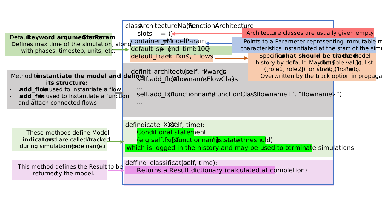
Click for full code template
class ArchitectureName(FunctionArchitecture): # Defining the class
    container_p = ParameterName # Attaching the parameter ParameterName to initialize at self.p
    default_sp = {‘end_time’: 100} # Set default values for the SimParam, in this case an end_time of 100 timesteps.
    default_track = [“fxns”, “flows] # Optionally we what to track, in this case "fxns" and "flows"

def init_architecture(self, **kwargs): # Method used to initialize the architecture by stitching functions and flows together
    self.add_flow(“outsideflowname”, FlowClass) # Always initialize the flows first.
    self.add_fxn(“functionname”, FunctionClass, “outsideflowname”) # Flows added next with the names of flows used in the function passed as arguments

def indicate_function_state_high(self): # optional conditional statement
    return self.fxns[“functionname”].s.varname2>200.0 # Note that these may be used to end the simulation when true if desired

def classify(self, scen={}, hists={}, **kwargs): # Method to classify results
    return {"combined_states": self.fxns["functionname"].s.varname1*self.fxns["functionname"].s.varname2} # In this case, this sends the same Result as the function class
There’s more to fmdtools than Functional Architectures {.smaller}
Often, resilience is about the complex interactions between operators/software/agents, infrastructure/the environment, and the physical system itself.
These systems-of-systems characteristics can also be modeled in fmdtools with the classes shown below:

These sorts of models are covered in Complex Systems Modeling in fmdtools
Demo Model Activity: {.smaller}
Open file:
For Pump example: examples/water_pump/model_main.py
For Drone example: examples/multirotor_drone/model_static.py
Notice the definitions and structure:
States - What variables are defined for what states or flows?
Modes - What modes are defined for what functions?
Flows - What flows are defined and what do they contain?
Functions - What functions are defined, what do they contain, and what are their behaviors?
FunctionArchitecture: - How do functions and flows connect in a model? How are results classified?
Parameter - What immutable variables are defined and for what functions/architectures?
Why do we structure models this way? {.smaller}
Enabling undirected propagation: Behavior from any Block in an Architecture can propagate to anything else, which is important for capturing the full set of hazardous behavior
Composability and Parameterization: OOP gives us the ability to create a number of co-existing model variants by varying parameters as well as creating sub-classes with different containers
Avoiding one big monolithic class: We can document and unit test individual simulation pieces a lot easier than one giant class, increasing code quality
More Resources for Model Definition {.smaller}
Note the docs for model definition are in https://nasa.github.io/fmdtools/docs-source/fmdtools.define.html
Other examples also can be helpful: https://nasa.github.io/fmdtools/examples/Examples.html
Notebook Activity: {.smaller}
Open tutorial_fmdtools_basics.ipynb:
Instantiate the model
mdl = Pump()ormdl = Drone()
Explore structure
Try different parameters!
Change things! What does the model directory look like?
dir(mdl)
simulate to given time with
mdl(time)
Simulation Concepts: Types of Simulations
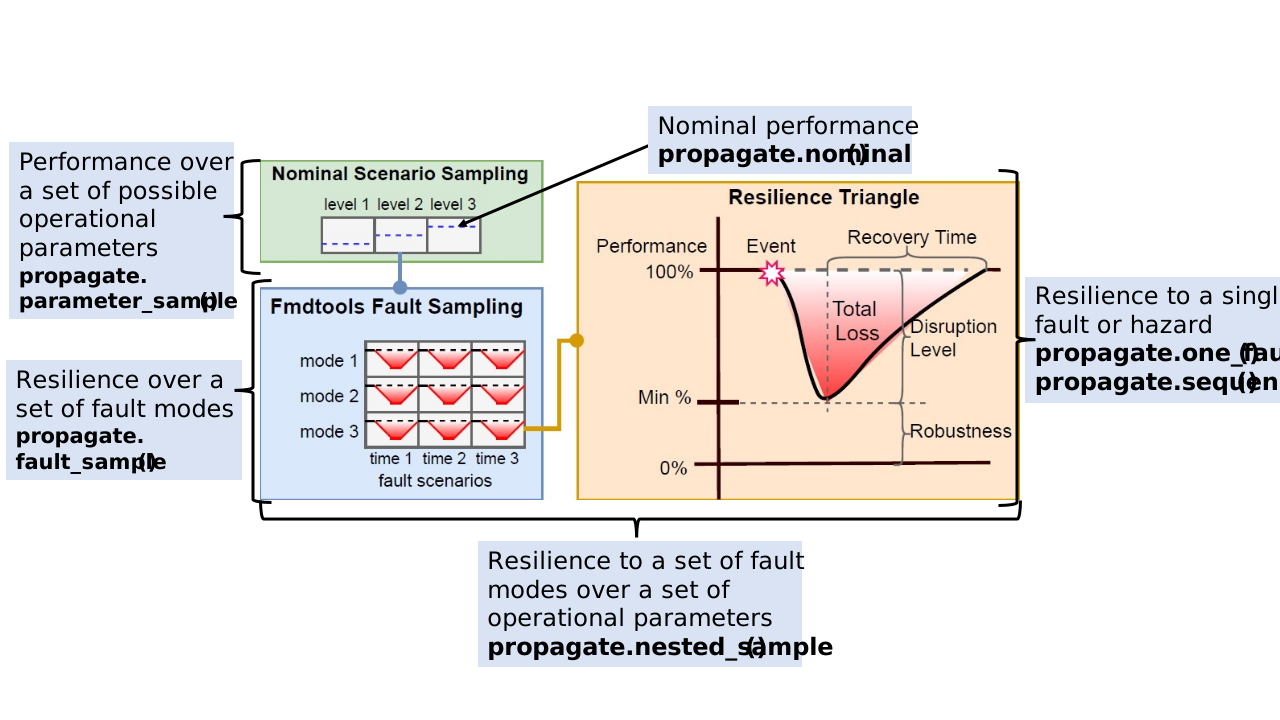
For more info on syntax/arguments, see documentation for fmdtools.sim.propagate.
Simulation Concepts: Sampling Approaches {.smaller}
These classes define multi-run simulations which can be used to quantify uncertain performance/resiliences:
SampleApproach/FaultSample: Which faults to sample and when
Relies on mode information encoded in the model
Simulated using
propagate.fault_sample()
ParameterSample: Nominal parameters or random seeds to sample
Can be simulated in
propagate.parameter_sample()Can be simulated in conjunction with faults using
propagate.nested_sample
See docs for: fmdtools.sim.fault_sample
Simulation Concepts: Things to Consider {.smaller}
Static/Dynamic propagation: How function states propagate to each other in a single time-step and multiple time-steps?
Stochastic Propagation: Whether and how stochastic states are instantiated over time - e.g. do we run with the “default” values of parameters, or do we sample from a random number generator?
Breadth of Scenarios: How hazards are represented as discrete scenarios to simulate - What set of joint faults do we use? How many times are sampled? - Operational scenarios and joint operational/fault scenarios
Activity: Simulate the Model {.smaller}
Run fault propagation methods: - propagate.nominal(), propagate.one_fault(), propagate.fault_sample()
What do the results look like? Explore data structures: - analyze.result.Result, analyze.result.History
Explore: - What happens when you change FaultSample parameters? - What happens when you change Model parameters? - How do these methods compare in terms of computational time?
Analysis Modules - see docs for fmdtools.analyze
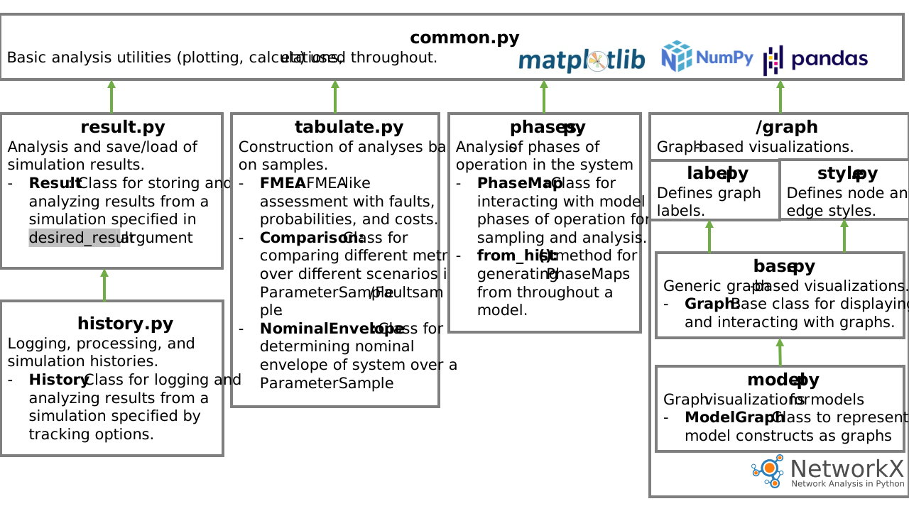
Analysis Activity {.smaller}
Visualize the results: - Show model graph - Show nominal performances - Show performances in a nominal scenario - Make a scenario-based FMEA
Explore: - How can you show only the parameters you want? Or change the formatting? - What does the behavior under other faults look like? - What other analyses can you perform with these results?
Starting your own repo/project {.smaller}
1.) Use uv init to create a template project, with its own virtual environment at .venv, README.md, and pyproject.toml files. - Fill in these files (e.g., fmdtools version, contributors, project description) - see: https://docs.astral.sh/uv/guides/projects/
2.) Install fmdtools into the venv: - uv pip install fmdtools or uv pip install fmdtools @ "./path/to/fmdtools"
3.) Set up the rest of the python tooling: https://github.com/nasa/fmdtools?tab=readme-ov-file#set-up-python-tooling-environment
5.) See if it all works! Get a script to run fmdtools from the venv kernel in your IDE.
6.) Commit and sync to remote
Conclusions/Summary {.smaller}
fmdtools is an environment for designing resilient systems
/defineenables model definition/simis used to define simulations/analyzeis used to analyze and visualize simulation results
I hope you agree that it has some powerful features!
Modeling expressiveness and clarity
Types of simulations that can be run
Powerful but easy-to-leverage plug-and-play analyses
Further Reading/Links {.smaller}
More advanced topics (see examples), including Search and optimization, Human, Systems-of-Systems modeling, and Modeling Stochastic Behavior
Model Development Best Practices: Has best practices for developing models in a strategic way (especially helpful for complex models)
Overview Paper: