Faulty State-Space Search Method Comparison

The goal of this notebook is to demonstrate the performance of evolutionary search methods on the hazard elicitation problem. The methods to compare are: - monte_carlo (a random search) - evolutionary algorithm - cooperative coevolutionary algorithm

These methods have been coded up using the deap simulation package in search_rover.py.

from search_rover import *
import pandas as pd

An experiment can be run calling the following methods:

result_mc, sol_mc= montecarlo(ngen=50, weight=0.5, filename='results/rslt_random.csv')
result_ea, sol_ea= ea(ngen=50, weight=0.5, filename='results/rslt_ea.csv')
result_ccea, sol_ccea, pop= ccea(ngen=50, weight=0.5, filename="results/rslt_ccea.csv")

MC PERFORMANCE:

100%|██████████████████████████████████████████████████████████████████████████████████| 50/50 [04:13<00:00,  5.06s/it]

Best Fitness: 0.44765907349504164
EA PERFORMANCE:

100%|██████████████████████████████████████████████████████████████████████████████████| 50/50 [04:44<00:00,  5.70s/it]

Best Fitness: 0.45991476941620624
CCEA PERFORMANCE:

100%|██████████████████████████████████████████████████████████████████████████████████| 50/50 [05:00<00:00,  6.00s/it]

Best Fitness: 0.5116345123278048

Alternatively, we can pull this data from saves:

dfrand = pd.read_csv('results/rslt_random.csv')
dfea = pd.read_csv('results/rslt_ea.csv')
dfccea = pd.read_csv("results/rslt_ccea.csv")

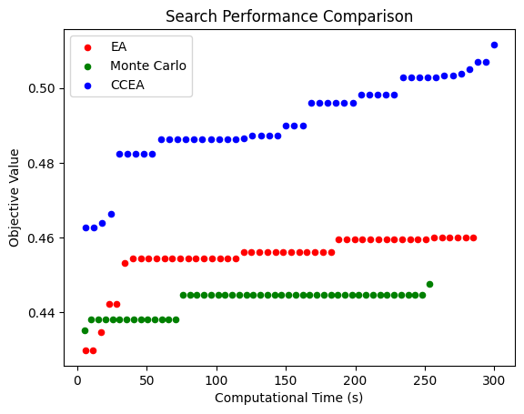
This shows the computational performance of (one run) of these methods:

# scatter plot
ax = dfea.plot(x='time', y= 'EA Fitness Values',c='r', kind='scatter', label='EA')
dfrand.plot(x='time', y='Random Fitness Values', kind='scatter', ax=ax, c='g', label='Monte Carlo')
dfccea.plot(x='time', y='CCEA Fitness Values', kind='scatter', ax=ax, c='b', label='CCEA')

# set the title

plt.ylabel("Objective Value")
plt.xlabel("Computational Time (s)")
plt.title("Search Performance Comparison")

C:\Users\dhulse\AppData\Roaming\Python\Python310\site-packages\pandas\plotting\_matplotlib\core.py:1258: UserWarning: No data for colormapping provided via 'c'. Parameters 'cmap' will be ignored
  scatter = ax.scatter(

Text(0.5, 1.0, 'Search Performance Comparison')

sol_ea = eval(dfea["EA Health States"].iloc[-1])
sol_mc = eval(dfrand["Random Health States"].iloc[-1])
sol_ccea = eval(dfccea["Best_Sol"].iloc[-1])
sols = {"Monte Carlo":sol_mc, "Evolutionary Algorithm":sol_ea, "Cooperative Coevolution":sol_ccea}

fig = plot_hspaces(sols)

---------------------------------------------------------------------------
AttributeError                            Traceback (most recent call last)
Cell In[6], line 1
----> 1 fig = plot_hspaces(sols)

File ~\Documents\GitHub\fmdtools\examples\rover\optimization\search_rover.py:672, in plot_hspaces(sol_dict, figsize, v_padding)
    670     k += 1
    671 ax = plt.gca()
--> 672 an.common.multiplot_legend_title.multiplot_legend_title(sol_dict, axs, ax, v_padding=v_padding)
    673 return fig

AttributeError: 'function' object has no attribute 'multiplot_legend_title'

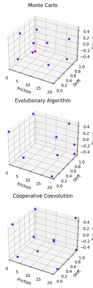
fig = plot_line_dist(sols)

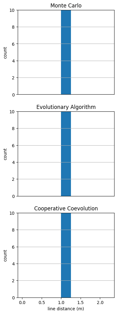
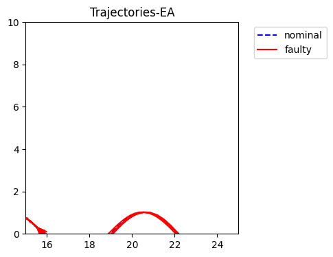
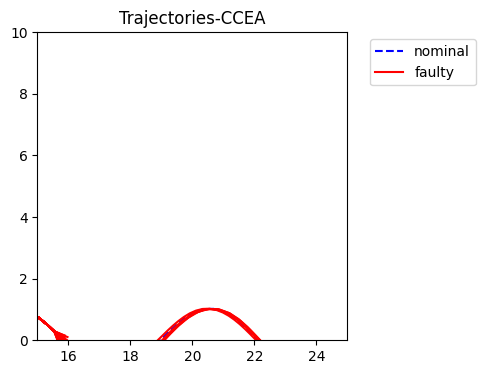
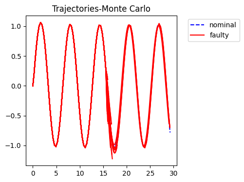
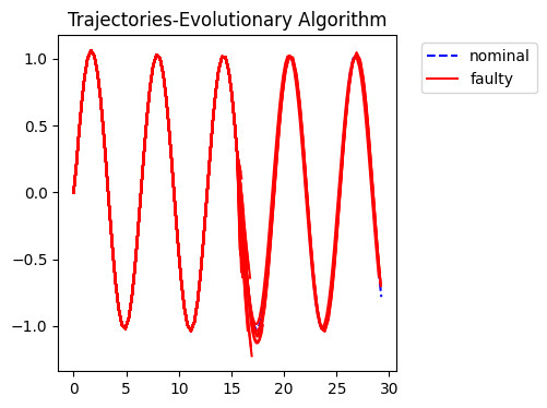
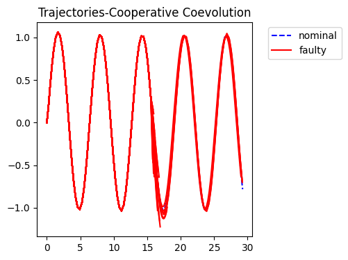
fig = plot_trajs(sols)

No artists with labels found to put in legend.  Note that artists whose label start with an underscore are ignored when legend() is called with no argument.

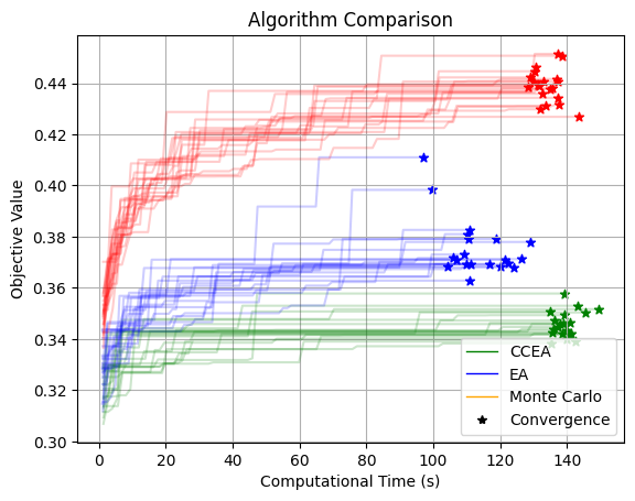
Performance Comparison

Comparing algorithm performance over 20 replicates, 100 (50 CCEA) generations, weight=0.5.

Estimated time = 3 mins * 3 types * 20 replicates = 180 minutes (3 hours).

num_replicates = 20

for i in range(num_replicates):
    result_mc, sol_mc= montecarlo(ngen=100, weight=0.5, filename="results/result_mc_"+str(i)+".csv", show_sol=False)
    result_ea, sol_ea= ea(ngen=100, weight=0.5, filename="results/result_ea_"+str(i)+".csv", show_sol=False)
    result_ccea, sol_ccea, pop= ccea(ngen=100, weight=0.5, filename="results/result_ccea_"+str(i)+".csv", show_sol=False)

MC PERFORMANCE:

  3%|██▍                                                                               | 3/100 [00:16<08:49,  5.46s/it]

---------------------------------------------------------------------------
KeyboardInterrupt                         Traceback (most recent call last)
Cell In[10], line 2
      1 for i in range(num_replicates):
----> 2     result_mc, sol_mc= montecarlo(ngen=100, weight=0.5, filename="results/result_mc_"+str(i)+".csv", show_sol=False)
      3     result_ea, sol_ea= ea(ngen=100, weight=0.5, filename="results/result_ea_"+str(i)+".csv", show_sol=False)
      4     result_ccea, sol_ccea, pop= ccea(ngen=100, weight=0.5, filename="results/result_ccea_"+str(i)+".csv", show_sol=False)

File ~\Documents\GitHub\fmdtools\examples\rover\optimization\search_rover.py:382, in montecarlo(verbose, ngen, show_sol, weight, filename, formulation)
    380 """Generate offspring"""
    381 offspring = toolbox.population()
--> 382 offspring = eval_pop_linedist(offspring)
    383 """Compute fitness values for all representative vectors.
    384 Assign representative fitness values to individuals that appeared in
    385 the representative vector. Assign max fitness from that array to be the
    386 individual fitness value. Using weighted sum to deal with multiple
    387 objectives"""
    388 for ind in offspring:

File ~\Documents\GitHub\fmdtools\examples\rover\optimization\search_rover.py:220, in eval_pop_linedist(pop)
    218 for k, ind in enumerate(pop):
    219     for i in range(len(ind)):
--> 220         ind[i].linedist, ind[i].enddist, ind[i].endpt = line_dist_faster(ind[i])
    221 return pop

File ~\Documents\GitHub\fmdtools\examples\rover\optimization\search_rover.py:57, in line_dist_faster(ind, show_plot, print_time)
     51 """
     52 Use Probleminterface class to calculate the same properties as line_dist.
     53
     54 (end dist, line dist, endpt)
     55 """
     56 starttime = time.time()
---> 57 dist = mode_search_prob.line_dist(*ind)
     58 end_dist = mode_search_prob.end_dist(*ind)
     59 endpt = [mode_search_prob.end_x(*ind), mode_search_prob.end_y(*ind)]

File c:\users\dhulse\documents\github\fmdtools\fmdtools\sim\search.py:182, in BaseProblem.add_objective_callable.<locals>.newobj(*x)
    181 def newobj(*x):
--> 182     return self.call_objective(*x, objective=name)

File c:\users\dhulse\documents\github\fmdtools\fmdtools\sim\search.py:245, in BaseProblem.call_objective(self, objective, *x)
    243 """Call a given objective at x."""
    244 if self.new_x(*x):
--> 245     self.update_objectives(*x)
    246 return self.objectives[objective].value

File c:\users\dhulse\documents\github\fmdtools\fmdtools\sim\search.py:599, in BaseSimProblem.update_objectives(self, *x)
    597 """Update objectives/constraints by simulating the model at x."""
    598 self.update_variables(*x)
--> 599 self.res, self.hist = self.sim_mdl(*x)
    600 for obj in {**self.objectives, **self.constraints}.values():
    601     if isinstance(obj, HistoryObjective) or isinstance(obj, HistoryConstraint):

File c:\users\dhulse\documents\github\fmdtools\fmdtools\sim\search.py:775, in ScenarioProblem.sim_mdl(self, *x)
    771     self.prep_sim()
    773 scen = self.gen_scenario(*x)
--> 775 mdl = [*self.prepped_sims['mdls'].values()][0].copy()
    776 nomhist = self.prepped_sims['hist'].copy()
    777 nomresult = self.prepped_sims['result'].copy()

File c:\users\dhulse\documents\github\fmdtools\fmdtools\define\architecture\base.py:337, in Architecture.copy(self, flows)
    335 # if flows provided from above, use those flows. Otherwise copy own.
    336 if hasattr(self, 'flows'):
--> 337     cargs['flows'] = {f: flows[f] if f in flows else obj.copy()
    338                       for f, obj in self.flows.items()}
    340 if hasattr(self, 'r'):
    341     cargs['r'] = self.r.copy()

File c:\users\dhulse\documents\github\fmdtools\fmdtools\define\architecture\base.py:337, in <dictcomp>(.0)
    335 # if flows provided from above, use those flows. Otherwise copy own.
    336 if hasattr(self, 'flows'):
--> 337     cargs['flows'] = {f: flows[f] if f in flows else obj.copy()
    338                       for f, obj in self.flows.items()}
    340 if hasattr(self, 'r'):
    341     cargs['r'] = self.r.copy()

File c:\users\dhulse\documents\github\fmdtools\fmdtools\define\environment.py:105, in Environment.copy(self, glob, p, s)
    103 cop.r.assign(self.r)
    104 cop.c = self.c.copy()
--> 105 cop.ga = self.ga.copy()
    106 if hasattr(self, 'h'):
    107     cop.h = self.h.copy()

File c:\users\dhulse\documents\github\fmdtools\fmdtools\define\architecture\base.py:342, in Architecture.copy(self, flows)
    340 if hasattr(self, 'r'):
    341     cargs['r'] = self.r.copy()
--> 342 cop = self.__class__(**cargs)
    343 cop.assign_roles('container', self)
    344 return cop

File c:\users\dhulse\documents\github\fmdtools\fmdtools\define\architecture\base.py:40, in Architecture.__init__(self, as_copy, h, *args, **kwargs)
     38 self._init_flexroles = []
     39 self.init_flexible_roles(**kwargs)
---> 40 self.init_architecture(**kwargs)
     41 self.build(**kwargs)

File c:\users\dhulse\documents\github\fmdtools\examples\rover\rover_model.py:229, in GroundGeomArch.init_architecture(self, **kwargs)
    227 """Initialize geometry with line and start/end points."""
    228 ls = self.p.gen_ls()
--> 229 self.add_line('line', PathLine, p={'xys': ls,
    230                                    'buffer_on': self.p.path_buffer_on,
    231                                    'buffer_poor': self.p.path_buffer_poor,
    232                                    'buffer_near': self.p.path_buffer_near})
    233 self.add_point('start', Dest, p={'x': ls[0][0], 'y': ls[0][1],
    234                                  'buffer_on': self.p.dest_buffer_on,
    235                                  'buffer_near': self.p.dest_buffer_near})
    236 self.add_point('end', Dest, p={'x': ls[-1][0], 'y': ls[-1][1],
    237                                'buffer_on': self.p.dest_buffer_on,
    238                                'buffer_near': self.p.dest_buffer_near})

File c:\users\dhulse\documents\github\fmdtools\fmdtools\define\architecture\geom.py:101, in GeomArchitecture.add_line(self, name, lclass, **kwargs)
     88 """
     89 Add/instantiate an individual line to the overall architecture.
     90
   (...)
     98     kwargs defining the object for gclass.
     99 """
    100 self.check_geom_class(lclass, GeomLine)
--> 101 self.add_flex_role_obj('lines', name, objclass=lclass, **kwargs)

File c:\users\dhulse\documents\github\fmdtools\fmdtools\define\architecture\base.py:105, in Architecture.add_flex_role_obj(self, flex_role, name, objclass, use_copy, **kwargs)
    102     as_copy = self.as_copy
    104 track = get_sub_include(name, get_sub_include(flex_role, self.track))
--> 105 obj = init_obj(name=name, objclass=objclass, track=track,
    106                as_copy=as_copy, **kwargs)
    108 if hasattr(obj, 'h') and obj.h:
    109     hist = obj.h

File c:\users\dhulse\documents\github\fmdtools\fmdtools\define\object\base.py:545, in init_obj(name, objclass, track, as_copy, **kwargs)
    543         fl.init_track(track)
    544     else:
--> 545         fl = objclass.copy(name=name, track=track, **kwargs)
    546 else:
    547     try:

File c:\users\dhulse\documents\github\fmdtools\fmdtools\define\object\geom.py:108, in Geom.copy(self, *args, **kwargs)
    106 def copy(self, *args, **kwargs):
    107     """Copy the Geom with given *args and **kwargs."""
--> 108     cop = self.__class__(*args, **kwargs)
    109     cop.s.assign(self.s)
    110     return cop

File c:\users\dhulse\documents\github\fmdtools\fmdtools\define\object\geom.py:49, in Geom.__init__(self, s, p, track, *args, **kwargs)
     47 def __init__(self, *args, s={}, p={}, track='default', **kwargs):
     48     super().__init__(s=s, p=p, track=[], **kwargs)
---> 49     self.shape = self.shapely_class(*self.p.as_args())
     50     # set buffer shapes
     51     self.init_role_dict("buffer")

File ~\AppData\Local\anaconda3\lib\site-packages\shapely\geometry\linestring.py:73, in LineString.__new__(self, coordinates)
     68 if len(coordinates) == 0:
     69     # empty geometry
     70     # TODO better constructor + should shapely.linestrings handle this?
     71     return shapely.from_wkt("LINESTRING EMPTY")
---> 73 geom = shapely.linestrings(coordinates)
     74 if not isinstance(geom, LineString):
     75     raise ValueError("Invalid values passed to LineString constructor")

File ~\AppData\Local\anaconda3\lib\site-packages\shapely\decorators.py:77, in multithreading_enabled.<locals>.wrapped(*args, **kwargs)
     75     for arr in array_args:
     76         arr.flags.writeable = False
---> 77     return func(*args, **kwargs)
     78 finally:
     79     for arr, old_flag in zip(array_args, old_flags):

File ~\AppData\Local\anaconda3\lib\site-packages\shapely\creation.py:120, in linestrings(coords, y, z, indices, out, **kwargs)
    118 coords = _xyz_to_coords(coords, y, z)
    119 if indices is None:
--> 120     return lib.linestrings(coords, out=out, **kwargs)
    121 else:
    122     return simple_geometries_1d(coords, indices, GeometryType.LINESTRING, out=out)

KeyboardInterrupt:

Loading results from saves:

dfs_mc, dfs_ea, dfs_ccea = [], [], []
for i in range(num_replicates):
    dfs_mc.append(pd.read_csv("results/result_mc_"+str(i)+".csv"))
    dfs_ea.append(pd.read_csv("results/result_ea_"+str(i)+".csv"))
    dfs_ccea.append(pd.read_csv("results/result_ccea_"+str(i)+".csv"))

Plotting results:

from matplotlib.lines import Line2D
dfs = [dfea, dfrand, dfccea]
for i, hist in enumerate(dfs_mc):
    plt.plot(hist['time'], hist['Random Fitness Values'], color='green', label="MC", alpha=0.2)
    plt.scatter(hist['time'].iloc[-1], hist['Random Fitness Values'].iloc[-1],  color='green', marker="*")
for i, hist in enumerate(dfs_ea):
    plt.plot(hist['time'], hist['EA Fitness Values'], color='blue', label="EA", alpha=0.2)
    plt.scatter(hist['time'].iloc[-1], hist['EA Fitness Values'].iloc[-1],  color='blue', marker="*")
for i, hist in enumerate(dfs_ccea):
    plt.plot(hist['time'], hist['CCEA Fitness Values'], color='red', label="CCEA", alpha=0.2)
    plt.scatter(hist['time'].iloc[-1], hist['CCEA Fitness Values'].iloc[-1],color='red', marker="*")
plt.legend()
ax = plt.gca()
handles, labels = ax.get_legend_handles_labels()
ax.get_legend().remove()
by_label = dict(zip(labels, handles))


legend_elements = [Line2D([0], [0], color='green', lw=1, label='CCEA'),
                   Line2D([0], [0], color='blue', lw=1, label='EA'),
                   Line2D([0], [0], color='orange', lw=1, label='Monte Carlo'),
                   Line2D([0], [0], marker='*', color='black', label='Convergence',
                          markerfacecolor='black',linestyle = 'None')]

ax.legend(handles=legend_elements)
#ax.legend(by_label.values(), by_label.keys(), prop={'size': 8})
plt.title("Algorithm Comparison")
plt.ylabel("Objective Value")
#plt.yscale("log")
plt.xlabel("Computational Time (s)")
plt.grid()
fig = plt.gcf()

mean_ea = np.mean([df['EA Fitness Values'] for df in dfs_ea],0)
times_ea = np.mean([df['time'] for df in dfs_ea],0)
std_ea = np.std([df['EA Fitness Values'] for df in dfs_ea],0)
mean_ccea = np.mean([df['CCEA Fitness Values'] for df in dfs_ccea],0)
times_ccea = np.mean([df['time'] for df in dfs_ccea],0)
std_ccea = np.std([df['CCEA Fitness Values'] for df in dfs_ccea],0)
mean_mc = np.mean([df['Random Fitness Values'] for df in dfs_mc],0)
times_mc = np.mean([df['time'] for df in dfs_mc],0)
std_mc = np.std([df['Random Fitness Values'] for df in dfs_mc],0)


plt.plot(times_ccea, mean_ccea, label="CCEA")
ax = plt.gca()
ax.fill_between(times_ccea,mean_ccea-std_ccea, mean_ccea+std_ccea, alpha=0.3)
plt.plot(times_ea, mean_ea, label="EA", linestyle='--')
ax.fill_between(times_ea,mean_ea-std_ea, mean_ea+std_ea, alpha=0.3)
plt.plot(times_mc, mean_mc, label="Monte Carlo", linestyle=':')
ax.fill_between(times_mc,mean_mc-std_mc, mean_mc+std_mc, alpha=0.3)
plt.legend()
plt.title("Search Performance ($\mu \pm \dfrac{\sigma}{2}$ over 20 Replicates)")
plt.ylabel("Objective Value")
#plt.yscale("log")
plt.xlabel("Computational Time (s)")
plt.grid()
fig = plt.gcf()
plt.xlim([0,207])
plt.ylim([0.5,1.06])
fig = plt.gcf()

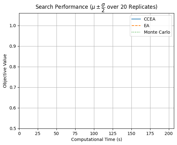
fig.savefig("alg_perf_comp.pdf", format="pdf", bbox_inches = 'tight', pad_inches = 0)

Comparing Solutions over weights - Fault-Space Formulation

Comparing results over weights given the goal is to explore the faulty state-space.

3 mins * 5 weights = 15 mins

weights = [0.0, 0.25, 0.5, 0.75, 1.0]

for i, w in enumerate(weights):
    result_ccea, sol_ccea, pop= ccea(ngen=100, weight=w, filename="results/result_weight_"+str(i)+".csv", show_sol=False)

Load Results

weight_sols = {}; weight_results = {}
for i, w in enumerate(weights):
    results = pd.read_csv("results/result_weight_"+str(i)+".csv")
    weight_sols["w="+str(w)] = eval(results["Best_Sol"].iloc[-1])

fig = plot_hspaces(weight_sols, v_padding=0.6)

fig.savefig("form1_fs_comp.pdf", format="pdf", bbox_inches = 'tight', pad_inches = 0)

fig = plot_line_dist(weight_sols)

fig.savefig("form1_ld_comp.pdf", format="pdf", bbox_inches = 'tight', pad_inches = 0)

fig = plot_trajs(weight_sols, v_padding=0.35)

fig.savefig("form1_traj_comp.pdf", format="pdf", bbox_inches = 'tight', pad_inches = 0)

line_dists = [sum([line_dist_faster(i)[0] for i in sol]) for sol in weight_sols.values()]

hs_dists = [f_2(sol) for sol in weight_sols.values()]

plt.scatter(line_dists, hs_dists, color='red')
for i,name in enumerate(weight_sols):
    plt.annotate(name, (line_dists[i], hs_dists[i]))
plt.xlabel("Sum of Line Distance")
plt.ylabel("Sum of Min Health State Separation")
plt.title("Revealed Pareto Front - Formulation 1")
plt.grid()
fig = plt.gcf()

fig.savefig("form1_fs_pareto.pdf", format="pdf", bbox_inches = 'tight', pad_inches = 0)

Multiplicative Formulation

result_ccea_1, sol_ccea_1, pop_1= ccea(ngen=100,  formulation=12, filename="results/result12_weight_.csv", show_sol=False)

visualizations(sol_ccea_1, method="CCEA-mult1")

fig=plot_hspace([sol_ccea_1])

linedists = [s.linedist for s in sol_ccea_1]
plt.hist(linedists, bins=[j for j in np.arange(0,2.5, 0.25)])
plt.title("CCEA-Mult1 Formulation")
plt.grid(axis="y")
plt.ylim([0,10])

line_dist_mult = f_1(sol_ccea_1)
point_dist_mult = f_2(sol_ccea_1)

plt.scatter(line_dists, hs_dists, color='blue')
for i,name in enumerate(weight_sols):
    plt.annotate(name, (line_dists[i], hs_dists[i]))
plt.xlabel("Sum of Line Distance")
plt.ylabel("Sum of Min Health State Separation")
plt.title("Pareto")
plt.grid()

plt.scatter([line_dist_mult], [point_dist_mult], color='red')
plt.annotate('mult', (line_dist_mult, point_dist_mult))
plt.xlabel("Sum of Line Distance")
plt.ylabel("Sum of Min Health State Separation")

As shown, the multiplicative formulation produces degenerate results, placing all weight on a single point instead of producing points that are both spread out and hazardous.

Comparing Solutions over weights - Result-Space Formulation

Comparing results over weights given the goal is to uncover new trajectories.

3 mins * 5 weights = 15 mins

weights = [0.0, 0.25, 0.5, 0.75, 1.0]

for i, w in enumerate(weights):
    result_ccea, sol_ccea, pop= ccea(ngen=100, weight=w, formulation=2, filename="results/result2_weight_"+str(i)+".csv", show_sol=False)

weight_sols = {}; weight_results = {}
for i, w in enumerate(weights):
    results = pd.read_csv("results/result2_weight_"+str(i)+".csv")
    weight_sols["w="+str(w)] = eval(results["Best_Sol"].iloc[-1])

fig = plot_hspaces(weight_sols, v_padding=0.6)

fig.savefig("form2_fs_comp.pdf", format="pdf", bbox_inches = 'tight', pad_inches = 0)

fig = plot_line_dist(weight_sols)

fig.savefig("form2_ld_comp.pdf", format="pdf", bbox_inches = 'tight', pad_inches = 0)

fig = plot_trajs(weight_sols, v_padding=0.35)

fig.savefig("form2_traj_comp.pdf", format="pdf", bbox_inches = 'tight', pad_inches = 0)

class ind(list):
    def __init__(self):
        self.endpt=[]

for w, sol in weight_sols.items():
    for index, i in enumerate(sol):
        new_i = ind()
        for j in i:
            new_i.append(j)
            new_i.endpt = line_dist_faster(i)[2]
        weight_sols[w][index]=new_i

line_dists = [sum([line_dist_faster(i)[0] for i in s]) for s in weight_sols.values()]
d_dists = [f_4(sol) for sol in weight_sols.values()]

plt.scatter(line_dists, d_dists, color='red')
for i,name in enumerate(weight_sols):
    plt.annotate(name, (line_dists[i], d_dists[i]))
plt.xlabel("Sum of Line Distance")
plt.ylabel("Sum of Min Result State Separation")
plt.title("Revealed Pareto Front - Formulation 2")
plt.grid()
fig = plt.gcf()

fig.savefig("form2_fs_pareto.pdf", format="pdf", bbox_inches = 'tight', pad_inches = 0)

result_ccea_2, sol_ccea_2, pop_2= ccea(ngen=100,  formulation=22, filename="results/result22_weight_.csv", show_sol=False)

visualizations(sol_ccea_2, method="CCEA-mult")

fig=plot_hspace([sol_ccea_2])

linedists = [s.linedist for s in sol_ccea_2]
plt.hist(linedists, bins=[j for j in np.arange(0,2.5, 0.25)])
plt.title("CCEA-Mult2 Formulation")
plt.grid(axis="y")
plt.ylim([0,10])

plt.scatter(line_dists, d_dists, color='red')
for i,name in enumerate(weight_sols):
    plt.annotate(name, (line_dists[i], d_dists[i]))
plt.xlabel("Sum of Line Distance")
plt.ylabel("Sum of Min Result State Separation")
plt.title("Pareto")
plt.grid()

line_dist_mult = f_1(sol_ccea_2)
point_dist_mult = f_4(sol_ccea_2)

plt.scatter(line_dists, d_dists, color='blue')
for i,name in enumerate(weight_sols):
    plt.annotate(name, (line_dists[i], d_dists[i]))
plt.xlabel("Sum of Line Distance")
plt.ylabel("Sum of Min Result State Separation")
plt.title("Pareto")
plt.grid()

plt.scatter([line_dist_mult], [point_dist_mult], color='red')
plt.annotate('mult', (line_dist_mult, point_dist_mult))
plt.xlabel("Sum of Line Distance")
plt.ylabel("Sum of Min Health State Separation")

As with the previous objective, the solutions produced appear degenerate in terms of objectives. Qualitatively, however, the results look “good” with both a wide range of trajectories and points with a high line distance.