

Visualize PACE-PAX Data#
Authors: Anna Windle (NASA, SSAI)
Adapted from code developed by: Ivona Cetinić (NASA, MSU), Kirk Knobelspiesse (NASA)
Last updated: October 28, 2026
The following notebooks are prerequisites for this tutorial.
Learn with OCI: Data Access
An Earthdata Login account is required to access data from the NASA Earthdata system, including NASA ocean color data.
Summary#
The PACE Postlaunch Airborne eXperiment (PACE-PAX) was a field campaign conducted in September 2024 in California and adjacent coastal areas. PACE-PAX brought together airborne and ship-based in situ observations to collect complementary atmospheric and oceanic measurements for the validation of observations from NASA’s PACE mission.
All PACE-PAX datasets are publicly available through the NASA Earthdata Cloud. This tutorial demonstrates how to access multiple PACE-PAX datasets, combine observations from different platforms, and create integrated visualizations to explore coupled atmosphere–ocean processes. This tutorial generates a multi-platform figure corresponding to Figure 9 in Knobelspiesse et al. (in review).
We will use the seabass-utils Python library to read in some of the PACE-PAX data. The SeaWiFS Bio-optical Archive and Storage System (SeaBASS) is a public archive of in situ oceanographic and atmospheric data maintained by the Ocean Biology Processing Group (OBPG) at NASA Goddard Space Flight Center (GSFC). seabass-utils is a collection of Python functions, also developed by the OBPG, to assist with SeaBASS data processing, file manipulation, and mapping tasks.
Learning Objectives#
At the end of this notebook you will be able to:
Access PACE-PAX datasets from the NASA Earthdata Cloud
Read and explore PACE-PAX datasets from SeaBASS
Combine observations from multiple platforms into a single data fusion visualization
Explore coupled atmosphere–ocean observations collected during PACE-PAX
1. Setup#
Begin by importing all of the packages used in this notebook. If you followed the guidance on the Getting-Started page, then the imports will be successful.
import cartopy.crs as ccrs
import earthaccess
import matplotlib.pyplot as plt
import pandas as pd
import plotly.graph_objects as go
import plotly.io as pio
import seabass_utils as sb
import xarray as xr
Set your Earthdata Login credentials. You can add persist=True to save your credentials in plain text in a netrc file, allowing you to authenticate automatically in the future sessions without re-entering your Earthdata credentials.
auth = earthaccess.login()
2. Access PACE-OCI data#
Let’s find a PACE-OCI Level-2 Inherent Optical Property (IOP) granule acquired during the PACE-PAX campaign over the Santa Barbara Channel, California. The IOP suite contains particulate backscattering data.
tspan = ("2024-09-26", "2024-09-26")
bbox = (-120, 33, -110, 35)
results = earthaccess.search_data(
short_name="PACE_OCI_L2_IOP",
temporal=tspan,
bounding_box=bbox,
)
len(results)
1
oci_paths = earthaccess.open(results)
We can open this file up using xarray and retrieve particulate backscattering at 442 nm data (bbp_442):
oci_dt = xr.open_datatree(oci_paths[-1])
oci_bbp = oci_dt["geophysical_data"]["bbp_442"]
for item in ("longitude", "latitude"):
oci_bbp[item] = oci_dt["navigation_data"][item]
oci_bbp
<xarray.DataArray 'bbp_442' (number_of_lines: 1710, pixels_per_line: 1272)> Size: 9MB
[2175120 values with dtype=float32]
Coordinates:
longitude (number_of_lines, pixels_per_line) float32 9MB ...
latitude (number_of_lines, pixels_per_line) float32 9MB ...
Dimensions without coordinates: number_of_lines, pixels_per_line
Attributes:
long_name: Particulate backscattering at 442 nm, GIOP model
units: m^-1
valid_min: -27999
valid_max: 2000
reference: P.J. Werdell, B.A. Franz, S.W. Bailey, G.C. Feldman and 15 c...
wavelength: 442.327Let’s subset the PACE-OCI bbp_442 data to a smaller geographical region in the Santa Barbara Channel, retain only positive values, and plot it:
subset = (
(oci_bbp["longitude"] >= -120.5)
& (oci_bbp["longitude"] <= -119.0)
& (oci_bbp["latitude"] >= 33.8)
& (oci_bbp["latitude"] <= 34.5)
)
oci_bbp = oci_bbp.where(subset & (oci_bbp >= 0), drop=True)
oci_bbp.sizes
Frozen({'number_of_lines': 79, 'pixels_per_line': 108})
crs = ccrs.PlateCarree()
fig, ax = plt.subplots(figsize=(8, 6), subplot_kw={"projection": crs})
oci_bbp.plot(
x="longitude",
y="latitude",
cmap="viridis",
vmax=0.015,
cbar_kwargs={"shrink": 0.65},
ax=ax,
)
ax.coastlines(resolution="10m", linewidth=1)
ax.gridlines(
draw_labels={"bottom": True, "left": True, "top": False, "right": False},
xlocs=plt.MaxNLocator(5),
ylocs=plt.MaxNLocator(5),
linewidth=0,
)
plt.tight_layout()
plt.show()
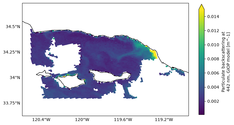
Higher bbp_442 values are observed along the coast, indicating greater particulate backscattering and potentially higher particle concentrations.
3. Access airborne optical data#
Now let’s access data collected from one of the aircraft flown during PACE-PAX. A Twin Otter airplane from the Center for Interdisciplinary Remotely Piloted Aircraft Studies (CIRPAS) at the Naval Postgraduate School in Monterey, CA, collected data on aerosol particles in the atmosphere. We will use the aerosol backscattering coefficient at 532 nm, measured under ambient relative humidity, temperature, and pressure, represented by the variable fine_amb_back_coef, produced by the In Situ Aerosol Retrieval Algorithm (ISARA).
results = earthaccess.search_data(
short_name="PACE-PAX_Analysis_ISARA_Data",
temporal=tspan,
)
len(results)
1
isara_paths = earthaccess.open(results)
isara_dt = xr.open_datatree(isara_paths[-1])
isara_bbp = isara_dt["derived"]["fine_amb_back_coef"].sel({"wavelength": 532})
for item in ("longitude", "latitude", "altitude"):
source_name = "GPS_Altitude_BUCHOLTZ" if item == "altitude" else f"{item.capitalize()}_BUCHOLTZ"
isara_bbp[item] = isara_dt["source"][source_name]
isara_bbp
<xarray.DataArray 'fine_amb_back_coef' (time: 691)> Size: 3kB
[691 values with dtype=float32]
Coordinates:
* time (time) float32 3kB 6.06e+04 6.063e+04 ... 8.127e+04 8.13e+04
longitude (time) float32 3kB ...
latitude (time) float32 3kB ...
altitude (time) float32 3kB ...
wavelength int32 4B 532
Attributes:
short_name: fine_amb_back_coef
units: Mm-1.sr-1
long_name: Backscattering coefficient at specified wavelength...
ACVSNC_standard_name: AerOpt_BackScattering_InSitu_BluetoRed_RHa_fine_AMBLet’s subset the data collected when the aircraft was flying in a spiral below 1 km:
subset = (
(isara_bbp["longitude"] >= -120.5)
& (isara_bbp["longitude"] <= -119.0)
& (isara_bbp["latitude"] >= 34.1)
& (isara_bbp["latitude"] <= 34.5)
& (isara_bbp["altitude"] <= 1000)
)
isara_bbp = isara_bbp.where(subset, drop=True)
isara_bbp.sizes
Frozen({'time': 105})
And use this to plot the flight track and vertical profile:
fig, axs = plt.subplots(1, 2, figsize=(10, 4))
cmap = plt.colormaps["plasma_r"].copy()
cmap.set_bad("gray")
sc1 = axs[0].scatter(
isara_bbp["longitude"],
isara_bbp["latitude"],
c=isara_bbp,
s=20,
cmap=cmap,
plotnonfinite=True,
)
axs[0].set_xlabel("Longitude")
axs[0].set_ylabel("Latitude")
axs[0].set_title("Twin Otter Flight Track")
axs[0].axis("equal")
sc2 = axs[1].scatter(
isara_bbp["longitude"],
isara_bbp["altitude"],
c=isara_bbp,
s=20,
cmap=cmap,
plotnonfinite=True,
)
axs[1].set_xlabel("Longitude")
axs[1].set_ylabel("Altitude")
axs[1].set_title("Twin Otter Vertical Profile")
fig.colorbar(
sc2,
ax=axs,
label=r"532 nm aerosol backscatter (Mm$^{-1}$ sr$^{-1}$)",
)
plt.show()
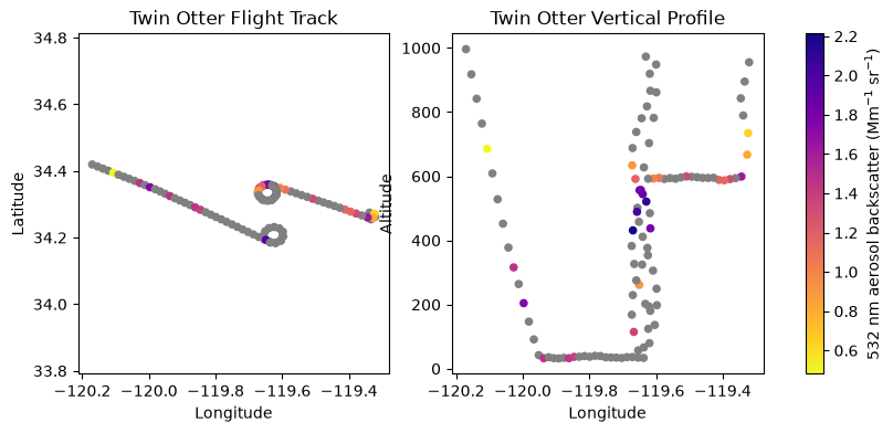
Note that the ISARA data are still being reprocessed, and ongoing changes may affect data validity and availability.
4. Access airborne lidar data#
The High Spectral Resolution Lidar 2 (HSRL-2) instrument was flown aboard NASA’s high altitude Earth Resources 2 (ER-2) aircraft to characterize atmospheric aerosol particles. We will use the aerosol backscatter coefficient measured at 532 nm.
We’ll open the file containing ‘R1’ indicating ‘Revision 1’, which contains the most up-to-date data.
results = earthaccess.search_data(
short_name="PACE-PAX_AircraftRemoteSensing_ER2_HSRL2_Data",
temporal=tspan,
granule_name="*R1*.h5",
)
len(results)
1
hsrl2_paths = earthaccess.open(results)
We will open this file using phony_dims='sort'. This is due to the NetCDF file containing groups or variables that reference dimensions that are not explicitly defined in the file. phony_dims='sort' creates phony dimensions in a sorted, more deterministic way to better reproduce NetCDF dimension behavior.
hsrl2_dt = xr.open_datatree(hsrl2_paths[-1], phony_dims='sort')
hsrl2_dt
<xarray.DataTree>
Group: /
│ Dimensions: (time: 2302, atime: 1, z: 1409)
│ Coordinates:
│ * time (time) datetime64[ns] 18kB 2024-09-26T16:58:42.403000 ... 2024-0...
│ * atime (atime) datetime64[ns] 8B 2024-09-26
│ * z (z) float64 11kB -500.0 -485.0 -470.0 ... 2.059e+04 2.061e+04
│ Data variables:
│ lat (time) float64 18kB ...
│ lon (time) float64 18kB ...
│ Attributes: (12/40)
│ ACVSNC_standard_name_URL: https://www-air.larc.nasa.gov/missions/etc...
│ ACVSNC_standard_name_version: 1.0
│ Conventions: CF-1.10
│ Format: HDF5
│ IdentifierProductDOI: 10.5067/ASDC/SUBORBITAL/PACE-PAX/DATA001/E...
│ PI_contact: Address: MS 401A NASA/LaRC, Hampton, VA 2...
│ ... ...
│ summary: PACEPAX Multiwavelength High Spectral Reso...
│ time_coverage_end: 2024-09-26 23:26:10
│ time_coverage_resolution: 10 s
│ time_coverage_start: 2024-09-26 16:58:42
│ title: PACEPAX Multiwavelength High Spectral Reso...
│ unit_convention: http://codes.wmo.int/wmdr/unit
├── Group: /DataProducts
│ Dimensions: (time: 2302, z: 1409, atime: 1,
│ phony_dim_3: 2302, phony_dim_4: 2,
│ phony_dim_5: 1, phony_dim_6: 1,
│ phony_dim_7: 1409)
│ Dimensions without coordinates: phony_dim_3, phony_dim_4, phony_dim_5,
│ phony_dim_6, phony_dim_7
│ Data variables: (12/71)
│ 1064_aer_dep (time, z) float64 26MB ...
│ 1064_aer_dep_cloud_screened (time, z) float64 26MB ...
│ 1064_aer_dep_syst_unc (time, z) float64 26MB ...
│ 1064_bsc (time, z) float64 26MB ...
│ 1064_bsc_Sa (time, z) float64 26MB ...
│ 1064_bsc_cloud_screened (time, z) float64 26MB ...
│ ... ...
│ Angstrom_Dust (time, z) float64 26MB ...
│ Angstrom_Spherical (time, z) float64 26MB ...
│ Dust_Mixing_Ratio (time, z) float64 26MB ...
│ WVD_1064_532 (time, z) float64 26MB ...
│ WVD_532_355 (time, z) float64 26MB ...
│ cloud_top_height (time, atime) float64 18kB ...
├── Group: /DataUncertainty
│ Dimensions: (time: 2302, z: 1409, atime: 1)
│ Data variables: (12/24)
│ 1064_aer_dep_cloud_screened_unc (time, z) float64 26MB ...
│ 1064_bsc_Sa_unc (time, z) float64 26MB ...
│ 1064_bsc_cloud_screened_unc (time, z) float64 26MB ...
│ 1064_dep_cloud_screened_unc (time, z) float64 26MB ...
│ 355_AOT_above_cloud_unc (time, atime) float64 18kB ...
│ 355_AOT_hi_col_unc (time, z) float64 26MB ...
│ ... ...
│ 532_bsc_Sa_unc (time, z) float64 26MB ...
│ 532_bsc_cloud_screened_unc (time, z) float64 26MB ...
│ 532_dep_cloud_screened_unc (time, z) float64 26MB ...
│ 532_ext_unc (time, z) float64 26MB ...
│ WVD_1064_532_unc (time, z) float64 26MB ...
│ WVD_532_355_unc (time, z) float64 26MB ...
├── Group: /Nav_Data
│ Dimensions: (phony_dim_8: 2302, phony_dim_9: 1)
│ Dimensions without coordinates: phony_dim_8, phony_dim_9
│ Data variables: (12/35)
│ Sday (phony_dim_8, phony_dim_9) float64 18kB ...
│ ambient_temp (phony_dim_8, phony_dim_9) float64 18kB ...
│ angle_of_attack (phony_dim_8, phony_dim_9) float64 18kB ...
│ cabin_press (phony_dim_8, phony_dim_9) float64 18kB ...
│ dew_point (phony_dim_8, phony_dim_9) float64 18kB ...
│ drift (phony_dim_8, phony_dim_9) float64 18kB ...
│ ... ...
│ use_wgs_for_gps (phony_dim_8, phony_dim_9) float64 18kB ...
│ vert_velocity (phony_dim_8, phony_dim_9) float64 18kB ...
│ vert_wind_speed (phony_dim_8, phony_dim_9) float64 18kB ...
│ wgs_alt (phony_dim_8, phony_dim_9) float64 18kB ...
│ wind_direction (phony_dim_8, phony_dim_9) float64 18kB ...
│ wind_speed (phony_dim_8, phony_dim_9) float64 18kB ...
├── Group: /State
│ Dimensions: (phony_dim_10: 2302, phony_dim_11: 1409,
│ phony_dim_12: 1, phony_dim_13: 1)
│ Dimensions without coordinates: phony_dim_10, phony_dim_11, phony_dim_12,
│ phony_dim_13
│ Data variables:
│ Number_Density (phony_dim_10, phony_dim_11) float64 26MB ...
│ O3 (phony_dim_10, phony_dim_11) float64 26MB ...
│ Pressure (phony_dim_10, phony_dim_11) float64 26MB ...
│ Relative_Humidity (phony_dim_10, phony_dim_11) float64 26MB ...
│ State_Type (phony_dim_12, phony_dim_13) float64 8B ...
│ Temperature (phony_dim_10, phony_dim_11) float64 26MB ...
│ U (phony_dim_10, phony_dim_11) float64 26MB ...
│ V (phony_dim_10, phony_dim_11) float64 26MB ...
│ Attributes:
│ source files: \nMERRA2_400.inst3_3d_asm_Np.20240926.SUB.nc\nMERRA2_400.i...
├── Group: /UserInput
│ Dimensions: (phony_dim_14: 1, phony_dim_15: 1,
│ phony_dim_16: 2302, phony_dim_17: 3,
│ phony_dim_18: 20, phony_dim_19: 1409)
│ Dimensions without coordinates: phony_dim_14, phony_dim_15, phony_dim_16,
│ phony_dim_17, phony_dim_18, phony_dim_19
│ Data variables: (12/60)
│ 1064_Sa_checkbox (phony_dim_14, phony_dim_15) float64 8B ...
│ 1064_attenbs_maxrange (phony_dim_14, phony_dim_15) float64 8B ...
│ 1064_attenbs_minrange (phony_dim_14, phony_dim_15) float64 8B ...
│ 1064_bs_range_avg (phony_dim_14, phony_dim_15) float64 8B ...
│ 1064_bs_time_avg (phony_dim_14, phony_dim_15) float64 8B ...
│ 1064_bsr_minimum_range (phony_dim_14, phony_dim_15) float64 8B ...
│ ... ...
│ lonGnd (phony_dim_16, phony_dim_14) float64 18kB ...
│ low_limit_checkbox (phony_dim_14, phony_dim_15) float64 8B ...
│ range50_interp (phony_dim_16, phony_dim_19) float64 26MB ...
│ range50_offset (phony_dim_14, phony_dim_15) float64 8B ...
│ range_interp (phony_dim_16, phony_dim_19) float64 26MB ...
│ range_offset (phony_dim_14, phony_dim_15) float64 8B ...
│ Attributes:
│ shiftValues120: [30. 30. 30. 30. 30. 30. 30. 30. 30. 30.]
│ shiftValues50: [19. 19. 19. 19.]
└── Group: /header
Dimensions: (phony_dim_20: 1, phony_dim_21: 1)
Dimensions without coordinates: phony_dim_20, phony_dim_21
Data variables:
LaserRepRate (phony_dim_20, phony_dim_21) float64 8B ...
N_Z (phony_dim_20, phony_dim_21) float64 8B ...
NumberBins (phony_dim_20, phony_dim_21) float64 8B ...
NumberChannels (phony_dim_20, phony_dim_21) float64 8B ...
SampleRate (phony_dim_20, phony_dim_21) float64 8B ...
aircraft (phony_dim_20, phony_dim_21) float64 8B ...
date (phony_dim_20, phony_dim_21) float64 8B ...
number_records (phony_dim_20, phony_dim_21) float64 8B ...We select the 532_bsc_cloud_screened variable and manually merge the auxiliary coordinates for longitude and latitude with the xarray.DataArray holding the backscatter coefficient.
hsrl2_bbp = hsrl2_dt["DataProducts"]["532_bsc_cloud_screened"]
for item in ("lon", "lat"):
hsrl2_bbp[item] = hsrl2_dt[item]
hsrl2_bbp
<xarray.DataArray '532_bsc_cloud_screened' (time: 2302, z: 1409)> Size: 26MB
[3243518 values with dtype=float64]
Coordinates:
* time (time) datetime64[ns] 18kB 2024-09-26T16:58:42.403000 ... 2024-0...
lon (time) float64 18kB ...
lat (time) float64 18kB ...
* z (z) float64 11kB -500.0 -485.0 -470.0 ... 2.059e+04 2.061e+04
Attributes: (12/14)
ACVSNC_standard_name: AerOpt_BackScattering_Profile_Green_RHa...
Comment: None
Horizontal resolution (seconds): 10.0
Horizontal_resolution_(seconds): 9.5
State source files: \nMERRA2_400.inst3_3d_asm_Np.20240926.S...
Vertical resolution (meters): 15.0
... ...
code_date: 13-Mar-2025
long_name: 532 nm aerosol backscatter coefficient ...
molecular depolarization: 0.0036
random_uncertainty: /DataUncertainty/532_bsc_cloud_screened...
run_date: 04-Apr-2025 16:21:59
units: km-1.sr-1We need to subset the data to a specific geographic location, altitude, and time. Both altitude and time are dimension coordinates, so we can extract the subset by slicing these coordinates. We restrict altitude from the surface to 1 km, and times within our time span of interest. This is a much reduced slice of the original data.
hsrl2_bbp = hsrl2_bbp.sel(
{
"time": slice("2024-09-26T19:32:24", "2024-09-26T19:38:24"),
"z": slice(0, 1000),
},
)
hsrl2_bbp.sizes
Frozen({'time': 37, 'z': 67})
Since we cannot slice on any auxiliary coordinates lacking an index, we must mask the backscatter coefficients for our geographic subsetting.
subset = (
(hsrl2_bbp["lon"] >= -120.2)
& (hsrl2_bbp["lon"] <= -119.0)
& (hsrl2_bbp["lat"] >= 34.1)
& (hsrl2_bbp["lat"] <= 34.5)
)
hsrl2_bbp = hsrl2_bbp.where(subset, drop=True)
hsrl2_bbp.sizes
Frozen({'time': 37, 'z': 67})
Now we are ready to visualize the lidar curtain as seen by the ER-2!
fig, ax = plt.subplots(figsize=(8, 4))
pcm = hsrl2_bbp.plot.imshow(
x="lon",
y="z",
cmap="inferno_r",
vmin=hsrl2_bbp.min(),
vmax=hsrl2_bbp.max(),
ax=ax,
cbar_kwargs={"label": "532 nm Backscatter [Mm$^{-1}$ sr$^{-1}$]"}
)
ax.set_xlabel("Longitude")
ax.set_title("HSRL-2 Aerosol Backscatter Curtain")
plt.show()
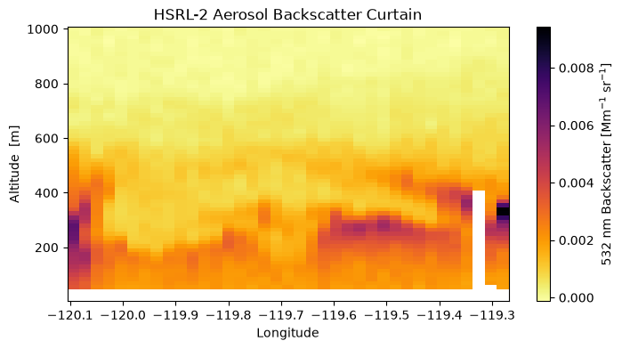
Notice higher aerosol backscatter at lower altitudes.
5. Access ship cast data#
In situ oceanic observations were collected aboard the NOAA R/V Shearwater. Particulate backscattering was measured using an SC6 backscattering sensor.
Let’s open the SC6 data collected on Sep 26th:
results = earthaccess.search_data(
short_name="PACE-PAX",
temporal=tspan,
granule_name="*Shearwater*SC6026*",
)
len(results)
4
These granules each reference multiple files containing data for that granule. At least one file for each granule is a plain .sb, rather than a .tgz.sb, indicating that it is a SeaBASS file.
urls = []
for item in results:
urls += [i for i in item.data_links() if not i.endswith(".tgz.sb")]
urls
['https://oceandata.sci.gsfc.nasa.gov/cmr/getfile/80370ff860_PACE-PAX_RV_Shearwater_SC6026_st38_R1.sb',
'https://oceandata.sci.gsfc.nasa.gov/cmr/getfile/80370ff860_PACE-PAX_RV_Shearwater_SC6026_st39_R1.sb',
'https://oceandata.sci.gsfc.nasa.gov/cmr/getfile/80370ff860_PACE-PAX_RV_Shearwater_SC6026_st40_R1.sb',
'https://oceandata.sci.gsfc.nasa.gov/cmr/getfile/80370ff860_PACE-PAX_RV_Shearwater_SC6026_st37_R1.sb']
sc6_paths = earthaccess.open(urls)
SeaBASS files can be read using the seabass_utils library, which we imported above as sb. The sb_read() function reads the SeaBASS file into a dictionary that pandas converts into a DataFrame.
Station information is extracted from header metadata and added as pandas.DataFrame columns:
sc6_bbp = []
for file in sc6_paths:
data = sb.sb_read(file, no_warn=True)
df = pd.DataFrame(data.data)
headers = data.headers
lat = float(headers["north_latitude"].split("[")[0])
lon = float(headers["east_longitude"].split("[")[0])
date = headers["start_date"]
time = headers["start_time"].split("[")[0]
bbp = df[["depth", "bbp440"]].assign(
**{
"date": date,
"time": time,
"latitude": lat,
"longitude": lon,
}
)
sc6_bbp.append(bbp)
sc6_bbp = pd.concat(sc6_bbp, ignore_index=True)
sc6_bbp.head()
| depth | bbp440 | date | time | latitude | longitude | |
|---|---|---|---|---|---|---|
| 0 | 0.4405 | 0.006945 | 20240926 | 16:41:02 | 34.1889 | -119.6281 |
| 1 | 0.9380 | 0.007183 | 20240926 | 16:41:02 | 34.1889 | -119.6281 |
| 2 | 1.9430 | 0.007060 | 20240926 | 16:41:02 | 34.1889 | -119.6281 |
| 3 | 2.8510 | 0.007014 | 20240926 | 16:41:02 | 34.1889 | -119.6281 |
| 4 | 4.1280 | 0.007370 | 20240926 | 16:41:02 | 34.1889 | -119.6281 |
And we can now plot the vertical profiles of particulate backscattering at 440 nm (bbp440):
fig, ax = plt.subplots(figsize=(5, 6))
sc = ax.scatter(
sc6_bbp["longitude"],
sc6_bbp["depth"],
c=sc6_bbp["bbp440"],
s=35,
cmap="viridis",
)
ax.invert_yaxis()
ax.set_xlabel("Longitude")
ax.set_ylabel("Depth (m)")
ax.set_title("R/V Shearwater SC6 $b_{bp}(440)$ profiles")
cbar = plt.colorbar(sc, ax=ax)
cbar.set_label("$b_{bp}(440)$ (m$^{-1}$)")
plt.tight_layout()
plt.show()
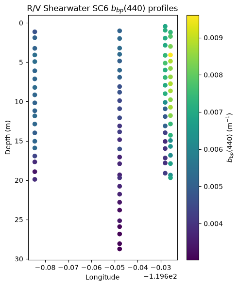
6. Access ocean glider data#
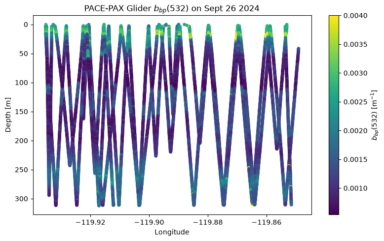
An autonomous ocean glider was also deployed along a 10 km transect for 25 days. The glider was equipped with a Seabird ECO Triplet optical sensor that measured particulate backscatter at 532 nm.
results = earthaccess.search_data(
short_name="PACE-PAX",
temporal=tspan,
granule_name="*glider*bbp*",
)
len(results)
1
eco_paths = earthaccess.open(results)
We will use sb.read() to open this data as well:
eco_data = sb.sb_read(eco_paths[0], no_warn=True)
eco_df = pd.DataFrame(eco_data.data)
eco_df.head()
| date | time | lat | lon | depth | wt | wt_sd | wt_bincount | cond | cond_sd | ... | bbp532_bincount | bbp700 | bbp700_sd | bbp700_bincount | bb532 | bb532_sd | bb532_bincount | bb700 | bb700_sd | bb700_bincount | |
|---|---|---|---|---|---|---|---|---|---|---|---|---|---|---|---|---|---|---|---|---|---|
| 0 | 20240907 | 21:23:10 | 34.26693 | -119.86806 | 0.155 | 17.3445 | 4.2924 | 106 | 45.0698 | 0.0107 | ... | 104 | 0.005235 | 0.001075 | 107 | 0.003669 | 0.000506 | 104 | 0.005540 | 0.001088 | 107 |
| 1 | 20240907 | 21:35:46 | 34.26700 | -119.87155 | 1.477 | 19.0290 | 0.0403 | 7 | 45.0329 | 0.0529 | ... | 7 | 0.004983 | 0.000242 | 7 | 0.003775 | 0.000131 | 7 | 0.005294 | 0.000242 | 7 |
| 2 | 20240907 | 21:35:52 | 34.26699 | -119.87159 | 2.503 | 18.4357 | 0.3851 | 6 | 44.3475 | 0.3927 | ... | 6 | 0.004860 | 0.000210 | 6 | 0.004545 | 0.000637 | 6 | 0.005171 | 0.000210 | 6 |
| 3 | 20240907 | 21:35:57 | 34.26699 | -119.87161 | 3.459 | 17.7523 | 0.0431 | 4 | 43.7660 | 0.0982 | ... | 4 | 0.004834 | 0.000109 | 4 | 0.004766 | 0.000540 | 4 | 0.005145 | 0.000109 | 4 |
| 4 | 20240907 | 21:36:02 | 34.26700 | -119.87162 | 4.482 | 17.4256 | 0.1180 | 5 | 43.4607 | 0.0818 | ... | 5 | 0.004660 | 0.000094 | 5 | 0.004438 | 0.000191 | 5 | 0.004971 | 0.000094 | 5 |
5 rows × 35 columns
Let’s filter out glider data for a specified date and location and keep only positive bbp532 values:
subset = (
(eco_df["date"] == 20240926)
& eco_df["lon"].between(-120.5, -119.0)
& eco_df["lat"].between(33.8, 34.5)
)
eco_bbp = eco_df.loc[subset & (eco_df["bbp532"] > 0)]
eco_bbp.shape
(12400, 35)
And we can plot bbp(532) along the glider’s track as it descended and ascended throughout the day:
fig, ax = plt.subplots(figsize=(8, 5))
sc = ax.scatter(
eco_bbp["lon"],
eco_bbp["depth"],
c=eco_bbp["bbp532"],
s=15,
cmap="viridis",
vmax=0.004,
)
ax.invert_yaxis()
ax.set_xlabel("Longitude")
ax.set_ylabel("Depth [m]")
ax.set_title("PACE-PAX Glider $b_{bp}(532)$ on Sept 26 2024")
cbar = plt.colorbar(sc, ax=ax)
cbar.set_label("$b_{bp}(532)$ [m$^{-1}$]")
plt.tight_layout()
plt.show()
7. Muli-platform Visualization#
In order to make all these data visually comparable, there are couple units discrepancies to smooth out. Ocean data use depth, which we’ll standardize to a “z” variable consistent with the altitude as used by airborne platforms. Both are in meters, just different conventions for positive.
sc6_bbp["z"] = -sc6_bbp["depth"]
eco_bbp["z"] = -eco_bbp["depth"]
The backscattering coefficients from the Twin Otter and ER-2 platforms are not the same units. We can convert the ER-2 platform’s data to units of Mm\(^{-1}\) sr\(^{-1}\) for plotting together.
hsrl2_bbp = hsrl2_bbp * 1000
hsrl2_bbp.attrs["units"] = "Mm-1.sr-1"
Now, we are able to show all this data together in one 3-dimensional plot:
pio.renderers.default = "notebook"
fig = go.Figure()
ocean_cmin = 0
ocean_cmax = 0.015
atmos_cmin = 0
atmos_cmax = 4
# --- PACE ---
fig.add_trace(
go.Surface(
x=oci_bbp["longitude"],
y=oci_bbp["latitude"],
z=oci_bbp.where(oci_bbp.isnull(), 0),
surfacecolor=oci_bbp,
colorscale="viridis",
showscale=True,
opacity=0.8,
cmin=ocean_cmin,
cmax=ocean_cmax,
colorbar={
"title": {
"text": "Ocean b<sub>bp</sub>(λ) [m⁻¹]",
"side": "right",
"font": {"size": 10},
},
"tickfont": {"size": 9},
"x": 0.8,
"y": 0.2,
"len": 0.4,
"tickvals": [0, 0.002, 0.004, 0.006, 0.008, 0.01],
"ticktext": ["0", "0.002", "0.004", "0.006", "0.008", "0.01"],
},
)
)
# --- Shearwater ---
fig.add_trace(
go.Scatter3d(
x=sc6_bbp["longitude"],
y=sc6_bbp["latitude"],
z=sc6_bbp["z"],
mode="markers",
marker={
"size": 3,
"color": sc6_bbp["bbp440"],
"colorscale": "viridis",
"showscale": False,
"cmin": ocean_cmin,
"cmax": ocean_cmax,
},
)
)
# --- Glider ---
fig.add_trace(
go.Scatter3d(
x=eco_bbp["lon"],
y=eco_bbp["lat"],
z=eco_bbp["z"],
mode="markers",
marker={
"symbol": "square",
"size": 3,
"color": eco_bbp["bbp532"],
"colorscale": "viridis",
"showscale": False,
"cmin": ocean_cmin,
"cmax": ocean_cmax,
},
line={"color": "lightgray", "width": 2},
)
)
# --- ER-2 ---
x, y, z, c = xr.broadcast(hsrl2_bbp["lon"], hsrl2_bbp["lat"], hsrl2_bbp["z"], hsrl2_bbp)
fig.add_trace(
go.Surface(
x=x,
y=y,
z=z.where(c.notnull()),
surfacecolor=c,
colorscale="inferno_r",
showscale=True,
cmin=atmos_cmin,
cmax=atmos_cmax,
colorbar={
"title": {
"text": "Aerosol b<sub>bp</sub>(532) [Mm⁻¹sr⁻¹]",
"side": "right",
"font": {"size": 10},
},
"tickfont": {"size": 9},
"x": 0.8,
"y": 0.6,
"len": 0.4,
},
)
)
# --- Twin Otter ---
fig.add_trace(
go.Scatter3d(
x=isara_bbp["longitude"],
y=isara_bbp["latitude"],
z=isara_bbp["altitude"],
mode="markers",
marker={
"size": 3,
"color": isara_bbp,
"colorscale": "plasma_r",
"showscale": False,
"cmin": atmos_cmin,
"cmax": atmos_cmax,
"line": {
"color": "black",
"width": 1,
},
},
)
)
fig.update_layout(
title={
"text": "Multi-Platform 3D Ocean/Atmosphere Visualization (Santa Barbara)",
"y": 0.995,
"yanchor": "top",
"x": 0.4,
"xanchor": "center",
},
scene={
"aspectmode": "manual",
"aspectratio": {"x": 1, "y": 1, "z": 0.8},
"xaxis": {"title": "Longitude", "range": [-120.2, -119.2]},
"yaxis": {"title": "Latitude", "range": [34.15, 34.45]},
"zaxis": {"title": "Height [m]", "range": [-400, 1000]},
"camera": {
"eye": {"x": -1.5, "y": -1.5, "z": 0.1}
},
},
width=1100,
height=800,
margin={"l": 0, "r": 100, "b": 200, "t": 0},
showlegend=False,
)
annotations_3d = [
{
"x": -120.1,
"y": 34.4,
"z": 5,
"text": "<b>PACE</b>",
"showarrow": False,
"font": {"size": 12, "color": "white"},
"bgcolor": "rgba(0,0,0,0.7)",
"borderpad": 4,
},
{
"x": -119.6,
"y": 34.22,
"z": -100,
"text": "<b>Shearwater</b>",
"showarrow": False,
"font": {"size": 12, "color": "blue"},
"bgcolor": "rgba(255,255,255,0.85)",
"borderpad": 4,
},
{
"x": -120.05,
"y": 34.3,
"z": -300,
"text": "<b>Glider</b>",
"showarrow": False,
"font": {"size": 12, "color": "green"},
"bgcolor": "rgba(255,255,255,0.85)",
"borderpad": 4,
},
{
"x": -119.6,
"y": 34.2,
"z": 800,
"text": "<b>Twin Otter</b>",
"showarrow": False,
"font": {"size": 12, "color": "purple"},
"bgcolor": "rgba(255,255,255,0.85)",
"borderpad": 4,
},
{
"x": -120.07,
"y": 34.41,
"z": 900,
"text": "<b>ER-2</b>",
"showarrow": False,
"font": {"size": 12, "color": "orange"},
"bgcolor": "rgba(255,255,255,0.85)",
"borderpad": 4,
},
]
fig.update_layout(scene={"annotations": annotations_3d})
fig.show()
You have completed the notebook on accessing and analyzing PACE-PAX data!