Exploring nitrogen dioxide (NO₂) data from PACE/OCI

Author(s): Anna Windle (NASA, SSAI), Zachary Fasnacht (NASA, SSAI)

Last updated: March 5, 2026

The following notebooks are prerequisites for this tutorial.

• File Structure (OCI Example)

An Earthdata Login account is required to access data from the NASA Earthdata system, including NASA ocean color data.

Summary

This tutorial describes how to access and download trace gas data products developed from PACE OCI data. More information on how these products were created can be found in Fasnacht et al. (2025). This notebook includes examples on how to plot L3M NO₂ data as a static and interactive map, as well as how to plot an interactive time series plot. It also provides examples on how to open and plot L2 NO₂ data.

Learning Objectives

At the end of this notebook you will know:

• How to access PACE OCI trace gas data products

• Where to find high NO₂ vertical column retrievals (hint: it’s a big city)

• How to create a time series of NO₂ data collected at a single location

• Open and plot L2 NO₂ data

1. Setup

Begin by importing all of the packages used in this notebook and setting your Earthdata Login credentials.

from datetime import datetime

import cartopy
import cartopy.crs as ccrs
import cartopy.feature as cfeature
import earthaccess
import holoviews
import hvplot.xarray
import matplotlib.colors
import matplotlib.pyplot as plt
import pandas as pd
import xarray as xr

holoviews.config.image_rtol = 1e-2

auth = earthaccess.login()

2. Search for L3M PACE Trace Gas Data

Level-2 (L2) and Level-3 mapped (L3M) trace gas (TRGAS) data products are available on NASA Earthdata.

Let’s search and open up the first L3M file collected during the temporal span of January 2025 to December 2025:

tspan = ("2025-01-01", "2025-12-31")

results = earthaccess.search_data(
    short_name="PACE_OCI_L3M_TRGAS",
    temporal=tspan,
    count=1,
)
paths = earthaccess.open(results)

paths

[<File-like object S3FileSystem, ob-cumulus-prod-public/PACE_OCI.20250101_20250131.L3m.MO.TRGAS.V3_0.0p1deg.nc>]

You can see that this search opened PACE_OCI.20250101_20250131.L3m.MO.TRGAS.V3_0.0p1deg.nc which is a L3M monthly (MO) composite with a 0.1° (0p1deg) pixel resolution.”

3. Open as an XArray dataset

We will use xarray.open_dataset to open the NetCDF and then merge them into a single dataset.

dataset = xr.open_dataset(paths[0])
dataset

<xarray.Dataset> Size: 52MB
Dimensions:           (lat: 1800, lon: 3600)
Coordinates:
  * lat               (lat) float32 7kB 89.95 89.85 89.75 ... -89.85 -89.95
  * lon               (lon) float32 14kB -179.9 -179.9 -179.8 ... 179.9 180.0
Data variables:
    total_column_o3   (lat, lon) float32 26MB ...
    total_column_no2  (lat, lon) float32 26MB ...
Attributes: (12/54)
    product_name:                      PACE_OCI.20250101_20250131.L3m.MO.TRGA...
    instrument:                        OCI
    title:                             OCI Level-3 Standard Mapped Image
    project:                           Ocean Biology Processing Group (NASA/G...
    platform:                          PACE
    source:                            satellite observations from OCI-PACE
    ...                                ...
    keywords:                          
    id:                                L3/PACE_OCI.20250101_20250131.L3m.MO.T...
    history:                           /sdps/sdpsoper/Science/OCSSW/V2026.2/b...
    processing_version:                3.0
    identifier_product_doi_authority:  https://dx.doi.org
    identifier_product_doi:            10.5067/PACE/OCI/L3M/TRGAS/3.0

xarray.Dataset

• Dimensions:
  • lat: 1800
  • lon: 3600
• Coordinates: (2)
  • lat
    (lat)
    float32
    89.95 89.85 89.75 ... -89.85 -89.95

    long_name :

    Latitude

    units :

    degrees_north

    standard_name :

    latitude

    valid_min :

    -90.0

    valid_max :

    90.0

    array([ 89.95    ,  89.85    ,  89.75    , ..., -89.75    , -89.850006,
           -89.950005], shape=(1800,), dtype=float32)

  • lon
    (lon)
    float32
    -179.9 -179.9 ... 179.9 180.0

    long_name :

    Longitude

    units :

    degrees_east

    standard_name :

    longitude

    valid_min :

    -180.0

    valid_max :

    180.0

    array([-179.95   , -179.85   , -179.75   , ...,  179.75   ,  179.85   ,
            179.95001], shape=(3600,), dtype=float32)

• Data variables: (2)
  • total_column_o3
    (lat, lon)
    float32
    ...

    long_name :

    Total vertical column ozone (O3)

    units :

    Dobson

    standard_name :

    atmosphere_mole_content_of_ozone

    valid_min :

    0.0

    valid_max :

    600.0

    display_scale :

    linear

    display_min :

    100.0

    display_max :

    500.0

    [6480000 values with dtype=float32]

  • total_column_no2
    (lat, lon)
    float32
    ...

    long_name :

    Total vertical column nitrogen dioxide (NO2)

    units :

    molecules cm^-2

    standard_name :

    atmosphere_mole_content_of_nitrogen_dioxide

    valid_min :

    0.0

    valid_max :

    1e+17

    display_scale :

    linear

    display_min :

    3e+15

    display_max :

    8e+15

    [6480000 values with dtype=float32]

• Attributes: (54)

  product_name :

  PACE_OCI.20250101_20250131.L3m.MO.TRGAS.V3_0.0p1deg.nc

  instrument :

  OCI

  title :

  OCI Level-3 Standard Mapped Image

  project :

  Ocean Biology Processing Group (NASA/GSFC/OBPG)

  platform :

  PACE

  source :

  satellite observations from OCI-PACE

  temporal_range :

  month

  time_coverage_start :

  2025-01-01T00:07:38.108Z

  time_coverage_end :

  2025-02-01T02:00:37.923Z

  start_orbit_number :

  0

  end_orbit_number :

  0

  map_projection :

  Equidistant Cylindrical

  latitude_units :

  degrees_north

  longitude_units :

  degrees_east

  northernmost_latitude :

  90.0

  southernmost_latitude :

  -90.0

  westernmost_longitude :

  -180.0

  easternmost_longitude :

  180.0

  geospatial_lat_max :

  90.0

  geospatial_lat_min :

  -90.0

  geospatial_lon_max :

  180.0

  geospatial_lon_min :

  -180.0

  latitude_step :

  0.1

  longitude_step :

  0.1

  sw_point_latitude :

  -89.95

  sw_point_longitude :

  -179.95

  spatialResolution :

  11.131949 km

  geospatial_lon_resolution :

  11.131949 km

  geospatial_lat_resolution :

  11.131949 km

  geospatial_lat_units :

  degrees_north

  geospatial_lon_units :

  degrees_east

  number_of_lines :

  1800

  number_of_columns :

  3600

  measure :

  Mean

  Conventions :

  CF-1.6 ACDD-1.3

  institution :

  NASA Goddard Space Flight Center, Ocean Ecology Laboratory, Ocean Biology Processing Group

  standard_name_vocabulary :

  CF Standard Name Table v36

  naming_authority :

  gov.nasa.gsfc.sci.oceandata

  license :

  https://science.nasa.gov/earth-science/earth-science-data/data-information-policy/

  creator_name :

  NASA/GSFC/OBPG

  publisher_name :

  NASA/GSFC/OBPG

  creator_email :

  data@oceancolor.gsfc.nasa.gov

  publisher_email :

  data@oceancolor.gsfc.nasa.gov

  creator_url :

  https://oceandata.sci.gsfc.nasa.gov

  publisher_url :

  https://oceandata.sci.gsfc.nasa.gov

  processing_level :

  L3 Mapped

  cdm_data_type :

  grid

  date_created :

  2026-06-05T18:35:05.091870Z

  keywords :

  id :

  L3/PACE_OCI.20250101_20250131.L3m.MO.TRGAS.V3_0.0p1deg.nc

  history :

  /sdps/sdpsoper/Science/OCSSW/V2026.2/bin/l3mapmerge -v l3mapmerge_inputs.txt PACE_OCI.20250101_20250131.L3m.MO.TRGAS.V3_0.0p1deg.nc [2026-06-05T18:35:11] ncattredit.py PACE_OCI.20250101_20250131.L3m.MO.TRGAS.V3_0.0p1deg.nc /tmp/PACE_OCI.20250101_20250131.L3m.MO.TRGAS.V3_0.0p1deg.nc.3809901

  processing_version :

  3.0

  identifier_product_doi_authority :

  https://dx.doi.org

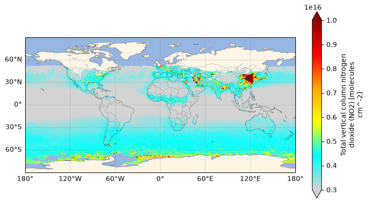
  identifier_product_doi :

  10.5067/PACE/OCI/L3M/TRGAS/3.0

If you expand the total_column_no2 variable, you’ll see that it is a 2D variable consisting of total vertical column NO₂ measurements with units of molecules cm^-2. Let’s plot it!

fig, ax = plt.subplots(figsize=(9, 5), subplot_kw={"projection": ccrs.PlateCarree()})
ax.coastlines(linewidth=0.2)
ax.add_feature(cfeature.BORDERS, linewidth=0.1)
ax.add_feature(cfeature.OCEAN, linewidth=0.2)
ax.add_feature(cfeature.LAKES, linewidth=0.2)
ax.add_feature(cfeature.LAND, facecolor="oldlace", linewidth=0.2)
cmap = matplotlib.colors.LinearSegmentedColormap.from_list(
    name="no2",
    colors=["lightgrey", "cyan", "yellow", "orange", "red", "darkred"],
)
dataset["total_column_no2"].plot(x="lon", y="lat", vmin=3e15, vmax=10e15, cmap=cmap)
ax.gridlines(
    draw_labels={"left": "y", "bottom": "x"},
    linewidth=0.25,
    color="grey",
    alpha=0.8,
)
plt.show()

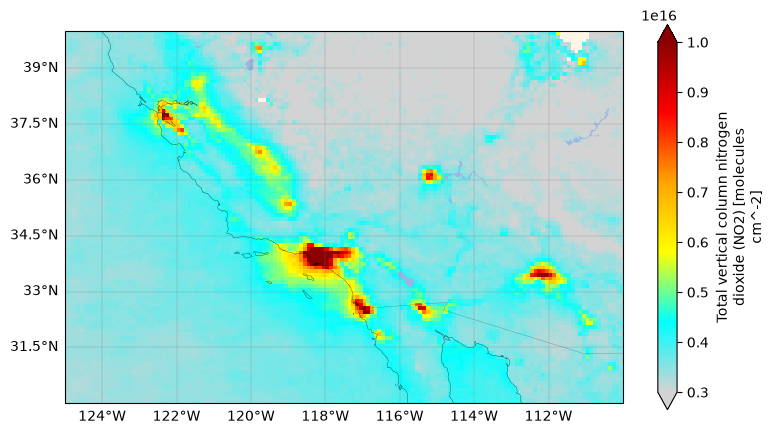
Let’s zoom in to Los Angeles, California.

plt.sca(ax)
plt.xlim(-125, -110)
plt.ylim(30, 40)
plt.show()

4. Interactive NO₂ plot

An interative plot allows you to engage with the data such as zooming, panning, and hovering over for more information. We will use the hvplot accessor on XArray data structures to make an interactive plot of the single file we accessed above.

dataset["total_column_no2"].hvplot(
    x="lon",
    y="lat",
    cmap=cmap,
    clim=(3e15, 10e15),
    aspect=2,
    title="Total vertical column NO₂ April 2024",
    widget_location="top",
    geo=True,
    coastline=True,
    tiles="EsriWorldStreetMap",
)