Explore HARP2 L2 V4.0 Land Products (FastMAPOL)

Explore HARP2 L2 V4.0 Land Products (FastMAPOL)#

Authors: Meng Gao (NASA/SSAI), Skye Caplan (NASA/SSAI)

Summary#

This notebook explores the HARP2 Level-2 (L2) land products generated by FastMAPOL. For more detailed information about the algorithm and data products, please refer to the FastMAPOL ATBD, including the data product list & land surface model.

You should already be familiar with exploring the FastMAPOL aerosol products from the other notebooks. Beginning with Version 4.0, FastMAPOL provides a new HARP2 aerosol and land surface product under the MAPOL_LAND data suite. This product is still undergoing evaluation and should be used with caution, as the retrievals may exhibit significant biases.

In this notebook, we focus on the retrieved land surface reflectance and its spectral and angular dependencies.

How to Cite#

If you use the PACE HARP2 MAPOL_LAND Version 4.0 data, please refer to the dataset information page for the latest citation and DOI:

https://www.earthdata.nasa.gov/data/catalog/ob-cloud-pace-harp2-l2-mapol-land-4.0

The dataset may be cited as:

NASA Ocean Biology Processing Group. (2026). PACE HARP2 Level-2 Regional Aerosol Over LAND Optical Properties, FastMAPOL Algorithm, Version 4.0. NASA Ocean Biology Distributed Active Archive Center (OB.DAAC). DOI: 10.5067/PACE/HARP2/L2/MAPOL_LAND/4.0. Accessed on: YYYY-MM-DD.

Learning Objectives#

By the end of this notebook, you will understand:

How to acquire HARP2 L2 data
What land surface products are available
How to visualize land surface reflectance
How to examine the angular dependence of surface reflectance and BRDF correction
How to evaluate basic retrieval quality metrics

1. Setup#

Begin by importing all the packages used in this notebook. If your kernel uses an environment defined following the guidance in the tutorials, the imports should be successful.

import math
from pathlib import Path

import earthaccess
import numpy as np
import pandas as pd
import xarray as xr

auth = earthaccess.login(persist=True)

4. Visualize HARP2 L2 Land Surface Properties#

In this example, we visualize the retrieved land surface reflectance. We first read the angular means and standard deviations before and after BRDF correction.

rhos_angular_mean = dataset["rhos_angular_mean"].values
rhos_angular_std = dataset["rhos_angular_std"].values

rhos_nadir_mean = dataset["rhos_nadir_mean"].values
rhos_nadir_std = dataset["rhos_nadir_std"].values

rhos_nadir_mean.shape

(395, 519, 4)

We also read the spatial coordinates and wavelength information.

lat = dataset["latitude"].values
lon = dataset["longitude"].values
plot_range = [lon.min(), lon.max(), lat.min(), lat.max()]
wavelength = dataset["wavelength"].values
wavelength

array([440.159, 549.465, 664.564, 865.283], dtype=float32)

Define helper functions for visualization#

The following helper functions are used to visualize single-band and RGB maps, examine the angular dependence of surface reflectance, and calculate reflectance ratios between selected viewing angles.

import matplotlib.pyplot as plt
from matplotlib.colors import LogNorm
import cartopy.crs as ccrs
import cartopy.feature as cfeature


def _prepare_rgba(data, vmin=None, vmax=None):
    """Normalize RGB/RGBA data and make invalid pixels transparent."""
    data = np.asarray(data, float)

    rgb = data[..., :3].copy()
    alpha = data[..., 3].copy() if data.shape[-1] == 4 else np.ones(data.shape[:2])

    valid = np.all(np.isfinite(rgb), axis=-1) & np.isfinite(alpha)

    if vmin is not None or vmax is not None:
        vmin1 = 0 if vmin is None else vmin
        vmax1 = np.nanmax(rgb) if vmax is None else vmax
        rgb = (rgb - vmin1) / (vmax1 - vmin1)

    rgb = np.clip(np.nan_to_num(rgb), 0, 1)
    alpha = np.where(valid, alpha, 0)

    return np.dstack([rgb, np.clip(alpha, 0, 1)])


def plot_l2_product(
    lon, lat, data, plot_range, label="", title="",
    vmin=None, vmax=None, figsize=(12, 4),
    cmap="viridis", log_scale=False,
    land_color="#f2efe9", ocean_color="#dbe9f6",
):
    """Plot scalar map + histogram, or RGB/RGBA map."""

    data = np.asarray(data)

    # Remove single-band dimension
    if data.ndim == 3 and data.shape[-1] == 1:
        data = data[..., 0]

    is_rgb = data.ndim == 3 and data.shape[-1] in (3, 4)

    # ---------------- Figure ----------------
    if is_rgb:
        fig, ax = plt.subplots(
            figsize=(figsize[0] * 0.75, figsize[1]),
            subplot_kw={"projection": ccrs.PlateCarree()},
        )

    else:
        if data.ndim != 2:
            raise ValueError("data must be 2D scalar or 3/4-band RGB.")

        values = data[np.isfinite(data)]
        if log_scale:
            values = values[values > 0]

        if values.size == 0:
            raise ValueError("No valid data.")

        vmin = np.percentile(values, 2) if vmin is None else vmin
        vmax = np.percentile(values, 98) if vmax is None else vmax

        fig = plt.figure(figsize=figsize)
        gs = fig.add_gridspec(1, 2, width_ratios=[3, 1], wspace=0.3)
        ax = fig.add_subplot(gs[0], projection=ccrs.PlateCarree())

    # ---------------- Background ----------------
    ax.set_extent(plot_range, crs=ccrs.PlateCarree())
    ax.add_feature(cfeature.OCEAN, facecolor=ocean_color, zorder=0)
    ax.add_feature(cfeature.LAND, facecolor=land_color, zorder=0)

    # ---------------- RGB ----------------
    if is_rgb:
        ax.pcolormesh(
            lon, lat, data,
            shading="nearest",
            transform=ccrs.PlateCarree(),
            zorder=1,
        )

    # ---------------- Scalar ----------------
    else:
        norm = LogNorm(vmin=vmin, vmax=vmax) if log_scale else None

        pm = ax.pcolormesh(
            lon, lat, data,
            cmap=cmap,
            norm=norm,
            vmin=None if log_scale else vmin,
            vmax=None if log_scale else vmax,
            shading="auto",
            transform=ccrs.PlateCarree(),
            zorder=1,
        )

        plt.colorbar(pm, ax=ax, pad=0.1).set_label(label)

        # Histogram
        axh = fig.add_subplot(gs[1])

        bins = (
            np.logspace(np.log10(vmin), np.log10(vmax), 40)
            if log_scale else 40
        )

        axh.hist(
            values,
            bins=bins,
            range=None if log_scale else (vmin, vmax),
            color="gray",
            edgecolor="black",
        )

        if log_scale:
            axh.set_xscale("log")

        axh.set(
            xlabel=label,
            ylabel="Count",
            title=f"Histogram: N={values.size}",
        )

    # ---------------- Decoration ----------------
    ax.coastlines(resolution="110m", linewidth=0.8, zorder=3)
    ax.gridlines(draw_labels=True, zorder=4)
    ax.set_title(title)

    plt.show()


########### Plot angular view for a pixel (or within a box)

def plot_rhos_angular(
    dataset, var, iy, ix, n=2,
    title=None, ylim=None
):
    rhos = dataset[var].values[..., 0]
    angle = dataset["sensor_view_angle"].values
    wv = dataset["intensity_wavelength"].values.squeeze()

    # Spatial mean/std
    box = rhos[iy-n:iy+n+1, ix-n:ix+n+1]
    mean = np.nanmean(box, axis=(0, 1))
    std = np.nanstd(box, axis=(0, 1))
    center = rhos[iy, ix]

    # Group by nominal wavelength
    wv_group = np.round(wv)
    wv_unique = np.unique(wv_group[np.isfinite(wv_group)])

    ncols = 2
    nrows = math.ceil(len(wv_unique) / ncols)

    fig, axes = plt.subplots(
        nrows, ncols,
        figsize=(10, 3.5*nrows),
        sharex=True
    )
    axes = np.atleast_1d(axes).ravel()

    for ax, wv1 in zip(axes, wv_unique):
        ind = wv_group == wv1
        order = np.argsort(angle[ind])

        a = angle[ind][order]
        m = mean[ind][order]
        s = std[ind][order]
        c = center[ind][order]

        ax.fill_between(a, m-s, m+s, alpha=0.25)
        ax.plot(a, m, "o-", label=f"{2*n+1}×{2*n+1} mean")
        ax.plot(a, c, "o--", label="Center pixel")

        ax.set_title(f"{wv1:.0f} nm")
        ax.set_xlabel("Sensor View Angle (°)")
        ax.set_ylabel(r"$\rho_s$")
        ax.grid(alpha=0.3)

        if ylim is not None:
            ax.set_ylim(ylim)

    # Remove unused panels
    for ax in axes[len(wv_unique):]:
        ax.remove()

    axes[0].legend()

    fig.suptitle(
        title or
        f"{var}\n"
        f"({dataset['latitude'].values[iy, ix]:.4f}°, "
        f"{dataset['longitude'].values[iy, ix]:.4f}°)"
    )

    plt.tight_layout()
    plt.show()


########### Compute ratios between two angles

def rhos_angle_ratio(dataset, var, iy, ix, angle1, angle2):
    rhos = dataset[var].values[..., 0]
    angle = dataset["sensor_view_angle"].values
    wv = np.round(dataset["intensity_wavelength"].values.squeeze())

    result = []

    for wv1 in np.unique(wv[np.isfinite(wv)]):
        ind = (wv == wv1)

        # Nearest observation within this wavelength band
        j1 = np.where(ind)[0][np.argmin(np.abs(angle[ind] - angle1))]
        j2 = np.where(ind)[0][np.argmin(np.abs(angle[ind] - angle2))]

        r1 = rhos[iy, ix, j1]
        r2 = rhos[iy, ix, j2]

        result.append([
            wv1,
            angle[j1],
            angle[j2],
            r1,
            r2,
            r2 / r1
        ])

    return pd.DataFrame(
        result,
        columns=[
            "wavelength",
            "angle1",
            "angle2",
            "rhos1",
            "rhos2",
            "ratio"
        ]
    )

Visualizations#

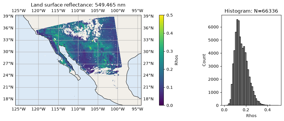
The following example shows land surface reflectance at a single wavelength. Note that rhos_nadir_mean represents the default reflectance to play with, which is the land surface reflectance after BRDF correction and nadir adjustment, followed by averaging over the available viewing angles per band.

wavelength_index = 1
title = "Land surface reflectance: " + str(wavelength[wavelength_index]) + " nm"
label = "Rhos"
data = rhos_nadir_mean[:, :, wavelength_index]

plot_l2_product(
    lon, lat, data,
    plot_range=plot_range,
    label=label,
    title=title,
    vmin=0,
    vmax=0.5,
    cmap="viridis"
)

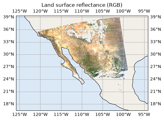
../../_images/3d3cc6666606cc525c3365f7ff0b7e10eb9b214b0ec9c6f3395b4b95e60faab8.png

The following example creates an RGB composite of the land surface reflectance. The selected bands are reordered from BGR to RGB, negative reflectances are clipped, and a gamma adjustment is applied for visualization.

# BGR -> RGB
data_rgb = rhos_nadir_mean[:, :, [2, 1, 0]].copy()

# Valid pixels
valid = np.all(np.isfinite(data_rgb), axis=-1)

# Gamma correction and scaling
data_rgb = np.clip(data_rgb, 0, None) ** 0.6
data_rgb = np.clip(data_rgb / 0.5, 0, 1)

# Add transparency
data_rgba = np.dstack([
    data_rgb,
    valid.astype(float),
])

plot_l2_product(
    lon,
    lat,
    data_rgba,
    plot_range=plot_range,
    title="Land surface reflectance (RGB)",
)

../../_images/a66f80eef676795c8fa34ba30e7edb494a956b8786b943e7760df304ed9112f0.png

5. Spectral Surface Reflectance#

The HARP2 land product also provides spectral information. Here, we examine a location near Railroad Valley at approximately 38.4958°N, 115.6964°W.

Find the center pixel#

The nearest HARP2 pixel to the target latitude and longitude is identified from the two-dimensional geolocation arrays.

lat_target = 38.4958
lon_target = -115.6964

dist2 = (lat - lat_target)**2 + (lon - lon_target)**2

iy, ix = np.unravel_index(np.nanargmin(dist2), dist2.shape)

print("Index:", iy, ix)
print("Lat/Lon:", lat[iy, ix], lon[iy, ix])

Index: 394 192
Lat/Lon: 36.775658 -115.321365

Extract the reflectance#

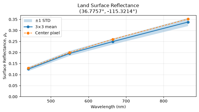
To explore the influence of pixel-to-pixel variability, we calculate the mean and standard deviation within a ±n-pixel neighborhood, corresponding to a (2n+1) × (2n+1) pixel box centered on the target location. The center-pixel reflectance is retained for comparison. The variability within the box can be used to assess the homogeneity of the surface properties.

rhos = dataset["rhos_nadir_mean"].values

# explore near by pixels
n = 1
npixel = 2*n+1

y0 = max(0, iy - n)
y1 = min(rhos.shape[0], iy + n + 1)

x0 = max(0, ix - n)
x1 = min(rhos.shape[1], ix + n + 1)

# shape: (ny, nx, wavelength)
rhos_box = rhos[y0:y1, x0:x1, :]

# Center pixel
rhos_target = rhos[iy, ix, :]

print("center pixel rhos:", rhos_target)

# Spatial statistics over the 5x5 neighborhood
rhos_mean = np.nanmean(rhos_box, axis=(0, 1))
rhos_std  = np.nanstd(rhos_box, axis=(0, 1))

print("average pixel rhos:", rhos_mean)

center pixel rhos: [0.12967816 0.19959638 0.2597795  0.3515005 ]
average pixel rhos: [0.12498599 0.19541222 0.2492357  0.3379093 ]

Plot the reflectance spectrum#

The figure compares the center-pixel spectrum with the 5 × 5 spatial mean. The shaded region represents ±1 standard deviation within the neighborhood.

plt.figure(figsize=(7, 4))

# Variation among neighboring pixels
plt.fill_between(
    wavelength,
    rhos_mean - rhos_std,
    rhos_mean + rhos_std,
    alpha=0.25,
    label=r"$\pm$1 STD"
)

# Neighborhood mean
plt.plot(
    wavelength, rhos_mean,
    "o-", lw=2,
    label=f"{npixel}×{npixel} mean"
)

# Center pixel
plt.plot(
    wavelength, rhos_target,
    "o--", lw=1.5,
    label="Center pixel"
)

plt.xlabel("Wavelength (nm)")
plt.ylabel(r"Surface Reflectance, $\rho_s$")
plt.title(
    f"Land Surface Reflectance\n"
    f"({lat[iy, ix]:.4f}°, {lon[iy, ix]:.4f}°)"
)

plt.ylim(bottom=0)
plt.grid(alpha=0.3)
plt.legend()
plt.tight_layout()
plt.show()

../../_images/07d6d405abbd95f8f30528dc02778b936744ce3a1f31db8d076d3d0068470a5e.png

6. Analyze the Angular Dependence#

The HARP2 land product preserves multi-angle information, allowing the angular dependence of the retrieved surface reflectance to be examined directly. Here, we again use the location near Railroad Valley.

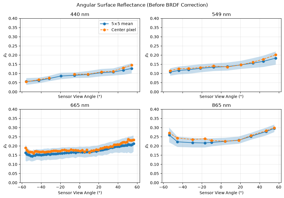
rhos_angular represents surface reflectance derived independently at each viewing angle before BRDF correction. The figure below shows the angular variation for each spectral band, together with the spatial variability within the 5 × 5 neighborhood.

plot_rhos_angular(
    dataset,
    "rhos_angular",
    iy, ix,
    title="Angular Surface Reflectance (Before BRDF Correction)",
    ylim=(0, 0.4)
)

../../_images/ea8e2d183899815f7c984011685d9ef476d355a66b44f8e54a5ed6e5b6d52cb0.png

We can also compare the surface reflectance at two selected viewing angles. The ratio between the two angles provides a simple measure of angular variation. Comparing this ratio among spectral bands can help assess whether the angular dependence is spectrally consistent.

The ratio reported below is defined as the reflectance at angle2 divided by the reflectance at angle1.

angle1, angle2 = 0, 30

ratio = rhos_angle_ratio(
    dataset,
    "rhos_angular",
    iy, ix,
    angle1=angle1,
    angle2=angle2
)

ratio

	wavelength	angle1	angle2	rhos1	rhos2	ratio
0	440.0	-5.29	35.040001	0.095634	0.111968	1.170801
1	549.0	6.60	33.220001	0.135480	0.161774	1.194085
2	665.0	0.60	30.180000	0.172352	0.192212	1.115228
3	865.0	4.20	31.070000	0.225939	0.256636	1.135868

The reverse ratio can be calculated by exchanging the two viewing angles.

angle1, angle2 = 30, 0

ratio = rhos_angle_ratio(
    dataset,
    "rhos_angular",
    iy, ix,
    angle1=angle1,
    angle2=angle2
)

ratio

	wavelength	angle1	angle2	rhos1	rhos2	ratio
0	440.0	35.040001	-5.29	0.111968	0.095634	0.854116
1	549.0	33.220001	6.60	0.161774	0.135480	0.837461
2	665.0	30.180000	0.60	0.192212	0.172352	0.896677
3	865.0	31.070000	4.20	0.256636	0.225939	0.880384

7. Angular Correction#

Angular correction is applied to rhos_angular to produce the nadir-adjusted surface reflectance, rhos_nadir. This remains an experimental product under evaluation.

Comparing rhos_nadir with rhos_angular provides a direct way to examine how the angular correction reduces the angular dependence of the retrieved surface reflectance.

plot_rhos_angular(
    dataset,
    "rhos_nadir",
    iy, ix,
    title="Angular Surface Reflectance (After BRDF Correction)",
    ylim=(0, 0.4)
)

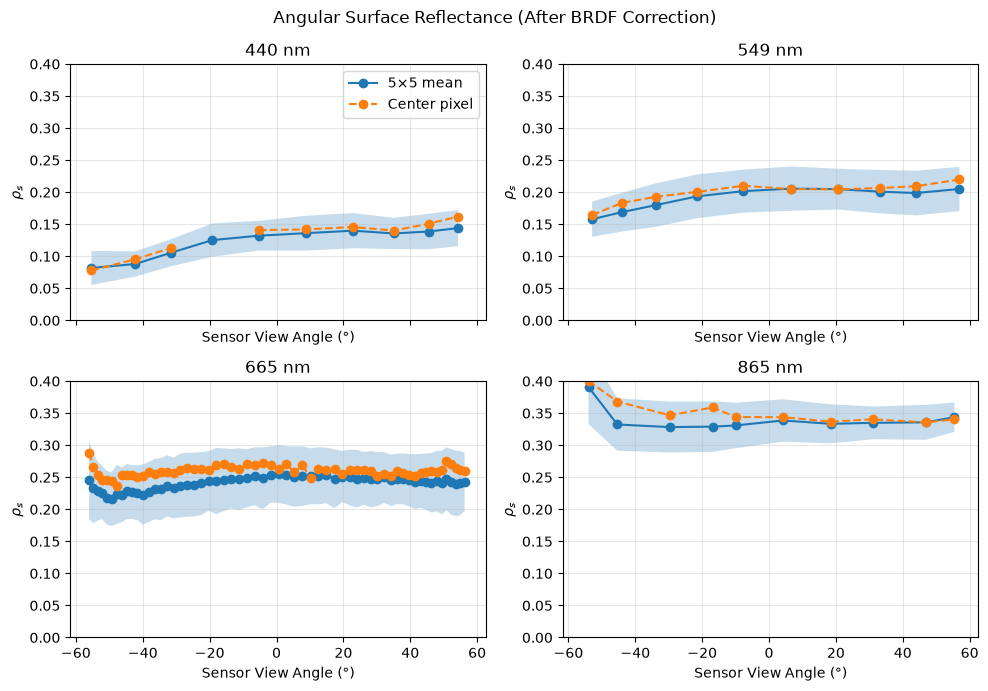
../../_images/3bb1814641d79631549a7a45a580470e9dc31b41a1c62872d5e765401bef175b.png

The reflectance ratios between selected viewing angles can also be recalculated using rhos_nadir. Ratios closer to unity after correction indicate reduced angular dependence.

angle1, angle2 = 0, 30

ratio = rhos_angle_ratio(
    dataset,
    "rhos_nadir",
    iy, ix,
    angle1=angle1,
    angle2=angle2
)

ratio

	wavelength	angle1	angle2	rhos1	rhos2	ratio
0	440.0	-5.29	35.040001	0.140894	0.140117	0.994483
1	549.0	6.60	33.220001	0.204868	0.206515	1.008040
2	665.0	0.60	30.180000	0.263601	0.252687	0.958598
3	865.0	4.20	31.070000	0.343762	0.340318	0.989983

angle1, angle2 = 30, 0

ratio = rhos_angle_ratio(
    dataset,
    "rhos_nadir",
    iy, ix,
    angle1=angle1,
    angle2=angle2
)

ratio

	wavelength	angle1	angle2	rhos1	rhos2	ratio
0	440.0	35.040001	-5.29	0.140117	0.140894	1.005548
1	549.0	33.220001	6.60	0.206515	0.204868	0.992024
2	665.0	30.180000	0.60	0.252687	0.263601	1.043190
3	865.0	31.070000	4.20	0.340318	0.343762	1.010118

For this example, the BRDF correction reduces a substantial portion of the angular variation, although residual angular dependence remains. The performance of this correction is still under evaluation.

8. Advanced: Quality Assessment#

As with the aerosol products, retrieval quality metrics are important for evaluating the land products, particularly when analyzing multi-angle information.

The primary metrics examined here are the retrieval cost function (chi2), the number of retained reflectance measurements (nv_ref), the number of retained DoLP (degree of linear polarization) measurements (nv_dolp), and the overall quality_flag. Please see the aerosol product tutorial or ATBD for more details.

chi2 = dataset["chi2"].values
nv_ref = dataset["nv_ref"].values
nv_dolp = dataset["nv_dolp"].values
quality_flag = dataset["quality_flag"].values

The retrieval cost function, \(\chi^2\), provides an overall measure of the agreement between the observations and the fitted forward model.

title = r"Retrieval cost function: $\chi^2$"
label = r"$\chi^2$"
data = chi2

plot_l2_product(
    lon, lat, data,
    plot_range=plot_range,
    label=label,
    title=title,
    vmin=0,
    vmax=3,
    cmap="viridis"
)

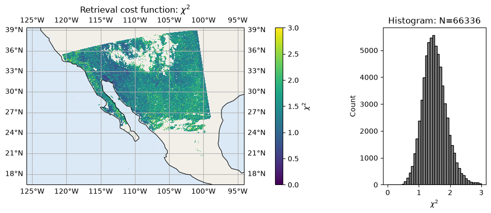
../../_images/aafa61811b75c8268b87a72506bd50601723e43e49434c119f1732c3cdd3342d.png

nv_ref gives the number of reflectance measurements retained in the retrieval.

title = r"Total number of reflectance measurements"
label = r"$N_{ref}$"
data = nv_ref

plot_l2_product(
    lon, lat, data,
    plot_range=plot_range,
    label=label,
    title=title,
    vmin=0,
    vmax=90,
    cmap="viridis"
)

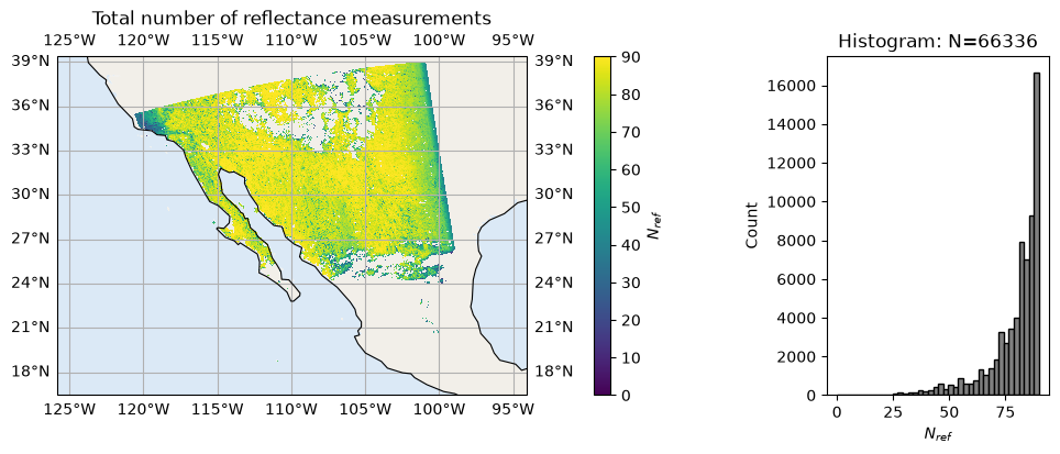
../../_images/986b24388bf34a4cc41c567fbbfafa71e47d84e62f2ec8078964a3e1a2e786b6.png

nv_dolp gives the number of DoLP measurements retained in the retrieval.

title = r"Total number of DoLP measurements"
label = r"$N_{dolp}$"
data = nv_dolp

plot_l2_product(
    lon, lat, data,
    plot_range=plot_range,
    label=label,
    title=title,
    vmin=0,
    vmax=90,
    cmap="viridis"
)

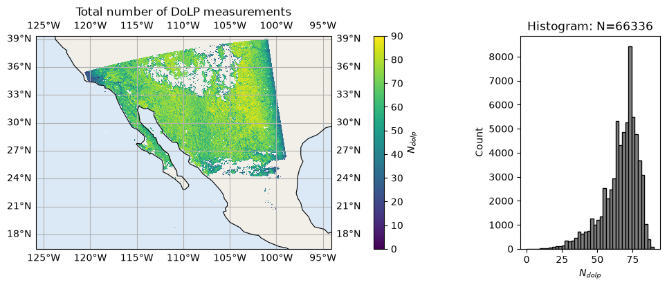
../../_images/a523cf29cb8e88a5a7ea8f0070c2b9042775ea5b10e3cba4acdc9e3481ef4e2b.png

The following provides simple granule-level averages of these retrieval metrics.

np.nanmean(chi2), np.nanmean(nv_ref), np.nanmean(nv_dolp)

(np.float32(1.5042068),
 np.float64(79.1215328027014),
 np.float64(66.33074047274481))

The overall retrieval quality is summarized by quality_flag.

The min and max value of the quality flags:

np.nanmin(data), np.nanmax(data)

(np.float64(10.0), np.float64(90.0))

title = "Retrieval quality flag"
label = "quality_flag"
data = quality_flag

plot_l2_product(
    lon, lat, data,
    plot_range=plot_range,
    label=label,
    title=title,
    vmin=0,
    vmax=6,
    cmap="viridis"
)

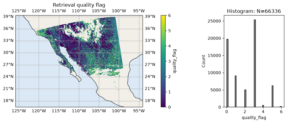
../../_images/1242a4ef8303c80721348e71b3ae8e7e1b5a87e0a838ccd465e101b2b42fdc71.png

The quality_flag is determined using retrieval metrics including \(\chi^2\) and the number of retained measurements. In this example, only a relatively small fraction of the retrievals, primarily near the center of the swath, meet the criteria for the highest-quality category (quality_flag = 0). Future improvements in instrument calibration and retrieval performance may increase the fraction of retrievals meeting the highest-quality criteria.

9. Advanced: Multi-Angle Data Mask#

To better understand the fitting and screening of individual angular measurements, we can examine the adaptive data masks.

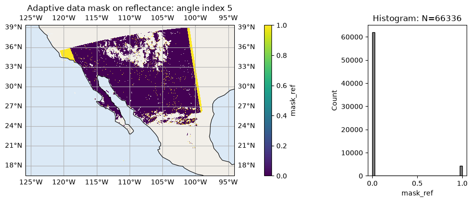
mask_ref indicates which reflectance measurements are retained or excluded during the retrieval, while mask_dolp provides the corresponding information for DoLP measurements.

mask_ref = dataset["mask_ref"].values
mask_dolp = dataset["mask_dolp"].values

mask_ref.shape, mask_dolp.shape

((395, 519, 90, 1), (395, 519, 90, 1))

The following example shows the reflectance data mask for one viewing-angle index.

angle_index = 5
title = "Adaptive data mask on reflectance: angle index " + str(angle_index)
label = "mask_ref"
data = mask_ref[:, :, angle_index, 0]

plot_l2_product(
    lon, lat, data,
    plot_range=plot_range,
    label=label,
    title=title,
    vmin=0,
    vmax=1,
    cmap="viridis"
)

../../_images/f6a0f99af298a089edce0c5336c5ff9a11ab79c67457314c10620ec603d4d314.png

The corresponding DoLP data mask can be examined in the same way.

angle_index = 5
title = "Adaptive data mask on DoLP: angle index " + str(angle_index)
label = "mask_DOLP"
data = mask_dolp[:, :, angle_index, 0]

plot_l2_product(
    lon, lat, data,
    plot_range=plot_range,
    label=label,
    title=title,
    vmin=0,
    vmax=1,
    cmap="viridis"
)

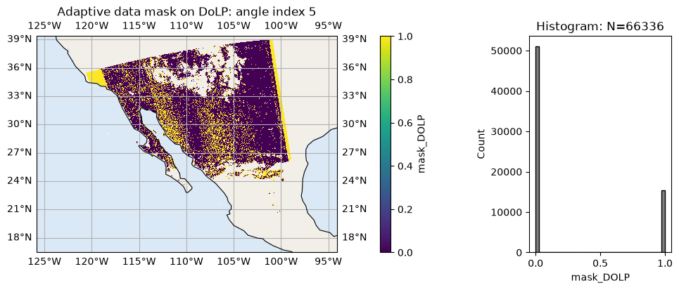
../../_images/e633f103122b4e47e09023b0ca5e21fadbf4038db79926ce47b59496c93bf2e8.png

Examining these masks for individual viewing angles can help identify where angular observations have been screened from the inversion.

10. References#

FastMAPOL ATBD.
[Algorithm] Gao, M., Franz, B. A., Zhai, P.-W., Knobelspiesse, K., Sayer, A. M., Xu, X., Martins, J. V., Cairns, B., Castellanos, P., Fu, G., Hannadige, N., Hasekamp, O., Hu, Y., Ibrahim, A., Patt, F., Puthukkudy, A., and Werdell, P. J.: Simultaneous retrieval of aerosol and ocean properties from PACE HARP2 with uncertainty assessment using cascading neural network radiative transfer models, Atmos. Meas. Tech., 16, 5863–5881, https://doi.org/10.5194/amt-16-5863-2023, 2023.