

Data Structure at Three Processing Levels for the Ocean Color Instrument (OCI)#
Author(s): Anna Windle (NASA, SSAI), Ian Carroll (NASA, UMBC), Carina Poulin (NASA, SSAI)
Last updated: July 14, 2026
The following notebooks are prerequisites for this tutorial.
An Earthdata Login account is required to access data from the NASA Earthdata system, including NASA ocean color data.
Summary#
In this example we will use the earthaccess package to access OCI Level-1B (L1B), Level-2 (L2), and Level-3-Mapped (L3M) NetCDF files and open them using xarray. While you can learn alot exploring the datasets in this way, be ready to refer to the full dataset documentation for details about the data products and processing.
NetCDF (Network Common Data Format) is a binary file format for storing multidimensional scientific data (variables). It is optimized for array-oriented data access and support a machine-independent format for representing scientific data. Files ending in .nc are NetCDF files.
XArray is a package that supports the use of multi-dimensional arrays in Python. It is widely used to handle Earth observation data, which often involves multiple dimensions — for instance, longitude, latitude, time, and channels/bands.
Learning Objectives#
At the end of this notebok you will know:
How to find groups in a NetCDF file
How to use
xarrayto open OCI dataWhat key variables are present in the groups within OCI L1B, L2, and L3M files
1. Setup#
Begin by importing all of the packages used in this notebook. If you followed the guidance on the Getting Started page, then the imports will be successful.
import cartopy.crs as ccrs
import earthaccess
import h5netcdf
import matplotlib.pyplot as plt
import numpy as np
import pandas as pd
import xarray as xr
Set your Earthdata Login credentials. You can add persist=True to save your credentials in a .netrc file, allowing you to authenticate automatically in the future sessions without re-entering your Earthdata credentials.
auth = earthaccess.login()
2. Explore L1B File Structure#
Let’s use xarray to open up a OCI L1B NetCDF file using earthaccess. We will use the same search method used in OCI Data Access. Note that L1B files do not include cloud coverage metadata, so we cannot use that filter.
tspan = ("2024-05-01", "2024-05-07")
bbox = (-76.75, 36.97, -75.74, 39.01)
results = earthaccess.search_data(
    short_name="PACE_OCI_L1B_SCI",
    temporal=tspan,
    bounding_box=bbox,
)
paths = earthaccess.open(results)
We want to know whether we are running code on a remote host with direct access to the NASA Earthdata Cloud. If without direct access, consider the substitution explained in the Data Access notebook to download granules.
If you see HTTPFileSystem in the output when you display paths, then earthaccess has determined that you do not have direct access to the NASA Earthdata Cloud.
Note, at present, it may be wrong.
Let’s open the first file of the L1B files list:
dataset = xr.open_dataset(paths[0])
dataset
<xarray.Dataset> Size: 0B
Dimensions:  ()
Data variables:
    *empty*
Attributes: (12/36)
    title:                             PACE OCI Level-1B Data
    instrument:                        OCI
    platform:                          PACE
    processing_level:                  L1B
    cdm_data_type:                     swath
    geospatial_lat_units:              degrees_north
    ...                                ...
    time_coverage_start:               2024-05-01T16:53:11.072Z
    time_coverage_end:                 2024-05-01T16:58:10.954Z
    processing_version:                3.0.2
    identifier_product_doi_authority:  https://dx.doi.org
    identifier_product_doi:            10.5067/PACE/OCI/L1B/SCI/3
history: 2026-05-07T14:16:40Z: l1bgen_oci ephfi...Notice that this xarray.Dataset has nothing but “Attributes”.
Instead of an xarray.Dataset, we want an xarray.DataTree to open NetCDF files that define more than one group of variable.
These “Groups” are almost equivalent to an xarray.Dataset, the difference is that a group can also contain another group!
datatree = xr.open_datatree(paths[0])
datatree
<xarray.DataTree>
Group: /
│   Attributes: (12/36)
│       title:                             PACE OCI Level-1B Data
│       instrument:                        OCI
│       platform:                          PACE
│       processing_level:                  L1B
│       cdm_data_type:                     swath
│       geospatial_lat_units:              degrees_north
│       ...                                ...
│       time_coverage_start:               2024-05-01T16:53:11.072Z
│       time_coverage_end:                 2024-05-01T16:58:10.954Z
│       processing_version:                3.0.2
│       identifier_product_doi_authority:  https://dx.doi.org
│       identifier_product_doi:            10.5067/PACE/OCI/L1B/SCI/3
│       history:                           2026-05-07T14:16:40Z: l1bgen_oci ephfi...
├── Group: /sensor_band_parameters
│       Dimensions:                (blue_bands: 119, red_bands: 163, SWIR_bands: 9,
│                                   HAM_sides: 2, polarization_coefficients: 3,
│                                   number_of_taps: 16)
│       Dimensions without coordinates: blue_bands, red_bands, SWIR_bands, HAM_sides,
│                                       polarization_coefficients, number_of_taps
│       Data variables: (12/16)
│           blue_wavelength        (blue_bands) float32 476B ...
│           blue_solar_irradiance  (blue_bands) float32 476B ...
│           red_wavelength         (red_bands) float32 652B ...
│           red_solar_irradiance   (red_bands) float32 652B ...
│           SWIR_wavelength        (SWIR_bands) float32 36B ...
│           SWIR_bandpass          (SWIR_bands) float32 36B ...
│           ...                     ...
│           red_m13_coef           (red_bands, HAM_sides, polarization_coefficients) float32 4kB ...
│           SWIR_m12_coef          (SWIR_bands, HAM_sides, polarization_coefficients) float32 216B ...
│           SWIR_m13_coef          (SWIR_bands, HAM_sides, polarization_coefficients) float32 216B ...
│           blue_spectral_mode     (number_of_taps) float32 64B ...
│           red_spectral_mode      (number_of_taps) float32 64B ...
│           SWIR_gain_type         (SWIR_bands) float32 36B ...
│       Attributes:
│           spatial_aggregation_factor:  8
├── Group: /scan_line_attributes
│       Dimensions:             (scans: 1710)
│       Dimensions without coordinates: scans
│       Data variables:
│           time                (scans) datetime64[ns] 14kB ...
│           spin_ID             (scans) float64 14kB ...
│           HAM_side            (scans) float32 7kB ...
│           scan_quality_flags  (scans) float32 7kB ...
├── Group: /geolocation_data
│       Dimensions:         (scans: 1710, pixels: 1272)
│       Coordinates:
│           latitude        (scans, pixels) float32 9MB ...
│           longitude       (scans, pixels) float32 9MB ...
│       Dimensions without coordinates: scans, pixels
│       Data variables:
│           height          (scans, pixels) float32 9MB ...
│           watermask       (scans, pixels) float32 9MB ...
│           sensor_azimuth  (scans, pixels) float64 17MB ...
│           sensor_zenith   (scans, pixels) float64 17MB ...
│           solar_azimuth   (scans, pixels) float64 17MB ...
│           solar_zenith    (scans, pixels) float64 17MB ...
│           quality_flag    (scans, pixels) float32 9MB ...
├── Group: /navigation_data
│       Dimensions:           (scans: 1710, quaternion_elements: 4, vector_elements: 3,
│                              pixels: 1272)
│       Dimensions without coordinates: scans, quaternion_elements, vector_elements,
│                                       pixels
│       Data variables:
│           att_quat          (scans, quaternion_elements) float32 27kB ...
│           att_ang           (scans, vector_elements) float32 21kB ...
│           orb_pos           (scans, vector_elements) float32 21kB ...
│           orb_vel           (scans, vector_elements) float32 21kB ...
│           sun_ref           (scans, vector_elements) float32 21kB ...
│           tilt_angle        (scans) float32 7kB ...
│           CCD_scan_angles   (scans, pixels) float32 9MB ...
│           SWIR_scan_angles  (scans, pixels) float32 9MB ...
├── Group: /observation_data
│       Dimensions:                 (blue_bands: 119, scans: 1710, pixels: 1272,
│                                    red_bands: 163, SWIR_bands: 9)
│       Dimensions without coordinates: blue_bands, scans, pixels, red_bands, SWIR_bands
│       Data variables:
│           rhot_blue               (blue_bands, scans, pixels) float32 1GB ...
│           rhot_red                (red_bands, scans, pixels) float32 1GB ...
│           rhot_SWIR               (SWIR_bands, scans, pixels) float32 78MB ...
│           qual_blue               (blue_bands, scans, pixels) float32 1GB ...
│           qual_red                (red_bands, scans, pixels) float32 1GB ...
│           qual_SWIR               (SWIR_bands, scans, pixels) float32 78MB ...
│           blue_percent_saturated  (blue_bands) float32 476B ...
│           red_percent_saturated   (red_bands) float32 652B ...
│           SWIR_percent_saturated  (SWIR_bands) float32 36B ...
│       Attributes:
│           striping_corrected:  yes
└── Group: /processing_control
    │   Attributes:
    │       software_name:     l1bgen_oci
    │       software_version:  Unspecified
    └── Group: /processing_control/input_parameters
            Attributes: (12/16)
                ifile:                PACE_OCI.20240501T165311.L1A.nc
                ofile:                PACE_OCI.20240501T165311.L1B.V3.nc
                cal_lut:              $OCVARROOT/oci/cal/OPER/PACE_OCI_L1B_LUT_V3_2026-04...
                geo_lut:              $OCVARROOT/oci/cal/OPER/PACE_OCI_GEO_LUT_2025-10-15.nc
                doi:
                crosstalk_lut:        $OCDATAROOT/oci/cal/PACE_OCI_cross_coef_LUT_2025-05...
                ...                   ...
                ephfile:              PACE_EPH_DEF_2024123_01.oem
                sline:                1
                eline:                -1
                enable_crosstalk:     false
                disable_aggregation:  false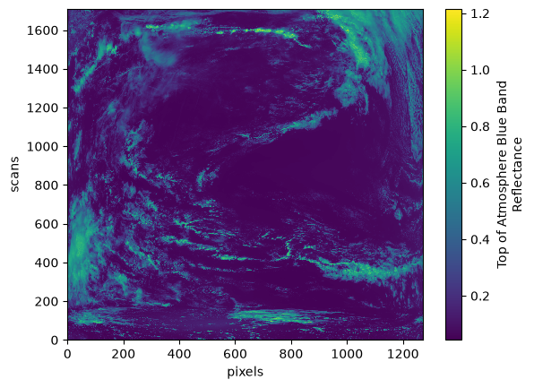
deflate: 5Now you can view the Dimensions, Coordinates, and Variables of each group. To show/hide any category, like “Groups”, toggle the drop-down arrow. To show/hide attributes, press the piece-of-paper icon on the right hand side of a variable. To show/hide data representation, press the stacked-cylinders icon. For instance, you could check the attributes on “rhot_blue” to see that this variable is the “Top of Atmosphere Blue Band Reflectance”.
The dimensions of the “rhot_blue” variable are (“blue_bands”, “number_of_scans”, “ccd_pixels”), as shown by the sizes attribute of the variable.
This gives us a dictionary of the array’s size in each dimension, keyed on the dimension names.
datatree["observation_data"]["rhot_blue"].sizes
Frozen({'blue_bands': 119, 'scans': 1710, 'pixels': 1272})
Let’s plot the reflectance at postion 100 in the “blue_bands” dimension.
plot = datatree["observation_data"]["rhot_blue"].sel({"blue_bands": 100}).plot()
3. Explore L2 File Structure#
OCI L2 files include retrievals of geophysical variables, such as Apparent Optical Properties (AOP), for each L1 swath. We’ll use the same earthaccess search for L2 AOP data. Although now we can use cloud_cover too.
clouds = (0, 50)
results = earthaccess.search_data(
    short_name="PACE_OCI_L2_AOP",
    temporal=tspan,
    bounding_box=bbox,
    cloud_cover=clouds,
)
paths = earthaccess.open(results)
Let’s look at the “geophysical_data” group, which is a new group generated by the level 2 processing, and the “Rrs” variable in particular.
datatree = xr.open_datatree(paths[-1])
rrs = datatree["geophysical_data"]["Rrs"]
rrs
<xarray.DataArray 'Rrs' (number_of_lines: 1709, pixels_per_line: 1272,
                         wavelength: 172)> Size: 1GB
[373901856 values with dtype=float32]
Coordinates:
  * wavelength  (wavelength) float32 688B 346.0 348.5 350.9 ... 716.8 719.3
Dimensions without coordinates: number_of_lines, pixels_per_line
Attributes:
    long_name:      Remote sensing reflectance
    units:          sr^-1
    standard_name:  surface_ratio_of_upwelling_radiance_emerging_from_sea_wat...
    valid_min:      -30000
valid_max: 25000The Rrs variable has 172 values in the wavelength; the blue, red, and SWIR wavelengths have been combined.
Without having to look too closely at the exact wavelength coordinates, we can plot the variable for a blue wavelength using method="nearest".
plot = rrs.sel({"wavelength": 440}, method="nearest").plot(cmap="viridis", robust=True)
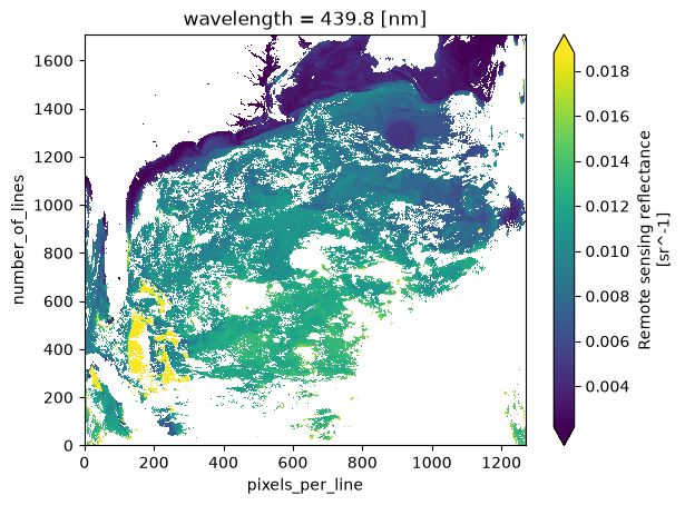
The scene is being plotted using number_of_lines and pixels_per_line as “x” and “y”, respectively.
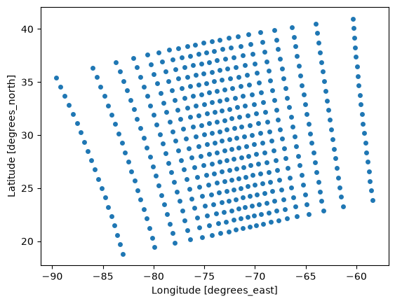
We need to add more coordinates, the latitude and longitude, for a true map.
These coordinates variables are in the “navigation_data” group.
for item in ("longitude", "latitude"):
    rrs[item] = datatree["navigation_data"][item]
rrs
<xarray.DataArray 'Rrs' (number_of_lines: 1709, pixels_per_line: 1272,
                         wavelength: 172)> Size: 1GB
[373901856 values with dtype=float32]
Coordinates:
    longitude   (number_of_lines, pixels_per_line) float32 9MB ...
    latitude    (number_of_lines, pixels_per_line) float32 9MB ...
  * wavelength  (wavelength) float32 688B 346.0 348.5 350.9 ... 716.8 719.3
Dimensions without coordinates: number_of_lines, pixels_per_line
Attributes:
    long_name:      Remote sensing reflectance
    units:          sr^-1
    standard_name:  surface_ratio_of_upwelling_radiance_emerging_from_sea_wat...
    valid_min:      -30000
valid_max: 25000Although we now have coordinates, they won’t immediately help because the data are not gridded by latitude and longitude.
L2 data come in the original instrument swath and have not been resampled to a regular grid.
That is why latitude and longitude are two-dimensional coordinates, and why the are not indexes like wavelength.
Latitude and longitude are present, but cannot be used immediately to look up values like you can with coordinates that are also indices.
Let’s make a scatter plot of some pixel locations so we can see the irregular spacing of latitude and longitude.
By selecting a slice with a step size larger than one, we get a subset of the locations for better visualization.
plot = datatree["navigation_data"].sel(
    {
        "number_of_lines": slice(None, None, 1720 // 20),
        "pixels_per_line": slice(None, None, 1272 // 20),
    },
).dataset.plot.scatter(x="longitude", y="latitude")
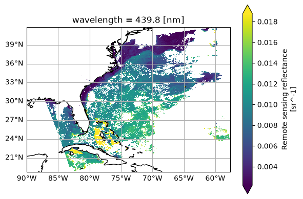
Despite not having indices, let’s plot Rrs the same way as before, except for the addition of latitude and longitude.
rrs_sel = rrs.sel({"wavelength": 440}, method="nearest")
plot = rrs_sel.plot(x="longitude", y="latitude", cmap="viridis", robust=True)

Plotting tools can handle non-index Coordinates! You can even visualize the data as if projected onto a grid. If you wanna get fancy, add a coastline.
fig, ax = plt.subplots(subplot_kw={"projection": ccrs.PlateCarree()})
im = rrs_sel.plot(x="longitude", y="latitude", cmap="viridis", robust=True, ax=ax)
ax.gridlines(draw_labels={"left": "y", "bottom": "x"})
ax.coastlines()
plt.show()
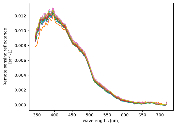
Let’s plot the full “Rrs” spectrum for individual pixels.
A visualization with all the pixels wouldn’t be useful, but limiting to a bounding box gives a simple way to subset pixels.
Note that, since we don’t have gridded data (i.e. our latitude and longitude coordinates are two-dimensional), we can’t slice on these values.
Without getting into anything complex, we will use a where with logical tests.
rrs_box = rrs.where(
    (
        (rrs["latitude"] > 26.0)
        & (rrs["latitude"] < 26.1)
        & (rrs["longitude"] > -84.1)
        & (rrs["longitude"] < -84.0)
    ),
    drop=True,
)
rrs_box.sizes
Frozen({'number_of_lines': 10, 'pixels_per_line': 3, 'wavelength': 172})
The line plotting method will only draw a line plot for 1D data, which we can get by stacking our two spatial dimensions and choosing to show the new “pixel dimension” in different hues.
rrs_stack = rrs_box.stack(
    {"pixel": ["number_of_lines", "pixels_per_line"]},
    create_index=False,
)
plot = rrs_stack.plot(hue="pixel", add_legend=False)
4. Explore L3M File Structure#
At L3M there are binned (B) and mapped (M) products available.
The L3M remote sensing reflectance (Rrs) files contain global maps of the full spectra, so they can be big!
We’ll use the same earthaccess method to find the data.
results = earthaccess.search_data(
    short_name="PACE_OCI_L3M_AOP",
    temporal=tspan,
)
len(results)
18
The L3M collections contain granules at different temporal and spatial resolutions. Let’s take a closer look at one of the larger sized granules first, using the metadata available on each result.
for item in results:
    if item.size() > 2000:
        display(item)
        break

Notice some special parts in the granule name:
Right after
L3myou have a period indicator. The valueDAYmeans a daily aggregate,8Dmeans an 8-day aggregate,MOmeans a monthly aggregate.Right before the
.ncsuffix, you have a spatial resolution marker. The value gives the horizontal cell size at the equator either in4kmor0p1deg. Readpas a decimal point.
Within a specific collection, earthaccess can retrieve granules whose name matches a pattern given in the granule_name argument.
Let’s use that to narrow our search to values aggregated to a month and 0.1 degree resolutions.
results = earthaccess.search_data(
    short_name="PACE_OCI_L3M_AOP",
    granule_name="*.MO.*.4km.*",
    temporal=tspan,
)
len(results)
1
paths = earthaccess.open(results)
L3M data do not have any groups, so we can open as a dataset rather than a datatree.
dataset = xr.open_dataset(paths[0])
dataset
<xarray.Dataset> Size: 26GB
Dimensions:     (lat: 4320, lon: 8640, wavelength: 172)
Coordinates:
  * lat         (lat) float32 17kB 89.98 89.94 89.9 ... -89.9 -89.94 -89.98
  * lon         (lon) float32 35kB -180.0 -179.9 -179.9 ... 179.9 179.9 180.0
  * wavelength  (wavelength) float32 688B 346.0 348.5 350.9 ... 716.8 719.3
Data variables:
    Rrs         (lat, lon, wavelength) float32 26GB ...
    nflh        (lat, lon) float32 149MB ...
    avw         (lat, lon) float32 149MB ...
    aot_865     (lat, lon) float32 149MB ...
    angstrom    (lat, lon) float32 149MB ...
Attributes: (12/55)
    product_name:                      PACE_OCI.20240501_20240531.L3m.MO.AOP....
    instrument:                        OCI
    title:                             OCI Level-3 Standard Mapped Image
    project:                           Ocean Biology Processing Group (NASA/G...
    platform:                          PACE
    source:                            satellite observations from OCI-PACE
    ...                                ...
    keywords:                          Earth Science > Oceans > Ocean Optics ...
    id:                                L3/PACE_OCI.20240501_20240531.L3m.MO.A...
    history:                           /sdps/sdpsoper/Science/OCSSW/V2026.2/b...
    processing_version:                3.2
    identifier_product_doi_authority:  https://dx.doi.org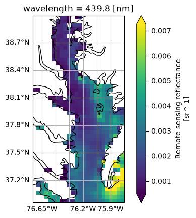
identifier_product_doi: 10.5067/PACE/OCI/L3M/OC_AOP/3.2Notice that this L3M granule has wavelength, lat, and lon under “Indexes”, so it’s easy to slice
out a bounding box and map the “Rrs” variable at a given wavelength.
rrs = dataset["Rrs"]
rrs_440_bbox = rrs.sel(
    wavelength=440, method="nearest").sel(
    lat=slice(bbox[3], bbox[1]),
    lon=slice(bbox[0], bbox[2]),
)
rrs_440_bbox
<xarray.DataArray 'Rrs' (lat: 49, lon: 24)> Size: 5kB
[1176 values with dtype=float32]
Coordinates:
  * lat         (lat) float32 196B 38.98 38.94 38.9 38.85 ... 37.06 37.02 36.98
  * lon         (lon) float32 96B -76.73 -76.69 -76.65 ... -75.85 -75.81 -75.77
    wavelength  float32 4B 439.8
Attributes:
    long_name:      Remote sensing reflectance
    units:          sr^-1
    standard_name:  surface_ratio_of_upwelling_radiance_emerging_from_sea_wat...
    valid_min:      -30000
    valid_max:      25000
    display_scale:  linear
    display_min:    0.0
display_max: 0.025fig, ax = plt.subplots(subplot_kw={"projection": ccrs.PlateCarree()})
im = rrs_440_bbox.plot(x="lon", y="lat", cmap="viridis", robust=True, ax=ax)
ax.gridlines(draw_labels={"left": "y", "bottom": "x"})
ax.coastlines()
plt.show()
Also becuase the L3M variables have gridded lat and lon coordinates, it’s possible to stack multiple granules along a new dimension that corresponds to time.
Using the granule_name filter, let’s get low spatial-resolution chlorophyll-a data to see daily changes.
results = earthaccess.search_data(
    short_name="PACE_OCI_L3M_BGC",
    temporal=tspan,
    granule_name="*.DAY.*.0p1deg.*",
)
print(len(results))

paths = earthaccess.open(results)
7
Instead of xr.open_dataset, we use xr.open_mfdataset to create a single xarray.Dataset (the “mf” in open_mfdataset stands for multiple files) from an array of paths.
The paths list is sorted temporally by default, which means the shape of the paths array specifies the way we need to tile the files together into larger arrays.
We specify combine="nested" to combine the files according to the shape of the array of files (or file-like objects), even though paths is not a “nested” list in this case.
The concat_dim="date" argument generates a new dimension in the combined dataset, because “date” is not an existing dimension in the individual files.
dataset = xr.open_mfdataset(
    paths,
    combine="nested",
    concat_dim="date",
)
Add a date variable as a coordinate using the dates from the netCDF files.
dates = [xr.open_dataset(i).attrs["time_coverage_end"] for i in paths]
dt = pd.to_datetime(dates)
dataset = dataset.assign_coords(date=dt.values)
dataset
<xarray.Dataset> Size: 726MB
Dimensions: (date: 7, lat: 1800, lon: 3600)
Coordinates:
* date (date) datetime64[us] 56B 2024-05-02T02:28:09.020000 ... 20...
* lat (lat) float32 7kB 89.95 89.85 89.75 ... -89.75 -89.85 -89.95
* lon (lon) float32 14kB -179.9 -179.9 -179.8 ... 179.8 179.9 180.0
Data variables:
poc (date, lat, lon) float32 181MB dask.array<chunksize=(1, 16, 1024), meta=np.ndarray>
pic (date, lat, lon) float32 181MB dask.array<chunksize=(1, 16, 1024), meta=np.ndarray>
chlor_a (date, lat, lon) float32 181MB dask.array<chunksize=(1, 16, 1024), meta=np.ndarray>
carbon_phyto (date, lat, lon) float32 181MB dask.array<chunksize=(1, 16, 1024), meta=np.ndarray>
Attributes: (12/55)
product_name: PACE_OCI.20240501.L3m.DAY.BGC.V3_2.0p1...
instrument: OCI
title: OCI Level-3 Standard Mapped Image
project: Ocean Biology Processing Group (NASA/G...
platform: PACE
source: satellite observations from OCI-PACE
... ...
keywords: Earth Science > Oceans > Ocean Chemist...
id: L3/PACE_OCI.20240501.L3m.DAY.BGC.V3_2....
history: /sdps/sdpsoper/Science/OCSSW/V2026.2/b...
processing_version: 3.2
identifier_product_doi_authority: https://dx.doi.org
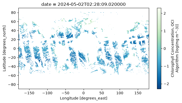
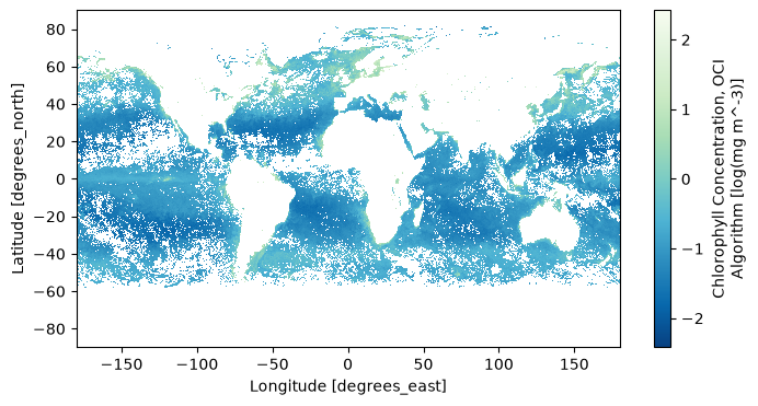
identifier_product_doi: 10.5067/PACE/OCI/L3M/OC_BGC/3.2A common reason to generate a single dataset from multiple, daily images is to create a composite. Compare the map from a single day …
chla = np.log10(dataset["chlor_a"])
chla.attrs.update(
    {
        "units": f'log({dataset["chlor_a"].attrs["units"]})',
    }
)
im = chla.sel(date="2024-05-02").plot(aspect=2, size=4, cmap="GnBu_r")
… to a map of average values, which ignore missing values due to clouds.
chla_avg = chla.mean("date", keep_attrs=True)
im = chla_avg.plot(aspect=2, size=4, cmap="GnBu_r")
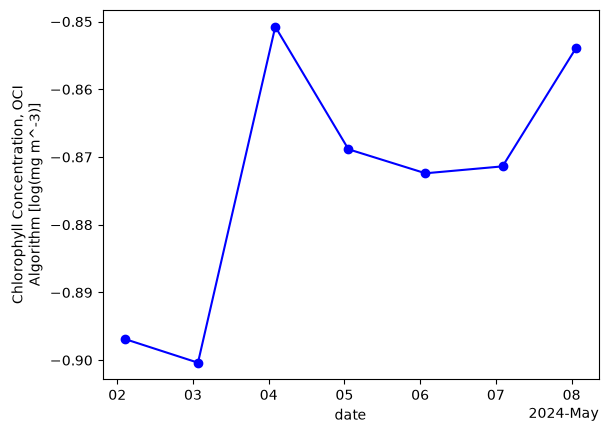
We can also create a time series of mean values over the whole region.
chla_avg = chla.mean(dim=["lon", "lat"], keep_attrs=True)
im = chla_avg.plot(linestyle="-", marker="o", color="b")
You have completed the notebook on OCI data structure. We now suggest reviewing the notebook on PACE OCI visualizations.