Visualize the PACE-OCI Level-2 CLOUD Products

Author(s): Chamara Rajapakshe (NASA, SSAI), Andy Sayer (NASA, UMBC), Kirk Knobelspiesse (NASA), Meng Gao (NASA, SSAI), Sean Foley (NASA, MSU)

Last updated: Oct 15, 2026

An Earthdata Login account is required to access data from the NASA Earthdata system, including NASA ocean color data.

Summary

This notebook summarizes how to access PACE-OCI cloud optical properties (CLOUD) in Level-2 (L2) granules. The CLOUD suite provides cloud optical and microphysical retrievals derived from multi-spectral observations. Note that this notebook is based on an early preliminary version of the product and is therefore subject to future optimizations and changes.

Learning Objectives

By the end of this notebook, you will understand:

• How to acquire PACE-OCI L2 CLOUD data

• Available variables in the CLOUD suite

• How to visualize cloud properties from PACE-OCI

1. Setup

Begin by importing all of the packages used in this notebook. If you followed the guidance on the Getting Started page, then the imports will be successful.

import re

import cartopy.crs as ccrs
import earthaccess
import matplotlib.colors as mcolors
import matplotlib.pyplot as plt
import numpy as np
import pandas as pd
import xarray as xr

Global settings and variables used throughout the notebook.

pd.options.display.max_colwidth = None
plt.style.use("seaborn-v0_8-notebook")
plt.rcParams.update(
    {
        "xtick.labelsize": 12,
        "ytick.labelsize": 12,
    }
)
projection = ccrs.PlateCarree()

Define your area and time of interest. Note that the bounding box is supplied as longitudes and latitudes in the order west, south, east, then north.

bbox = (-90, -13, -89, -12)
tspan = ("2025-07-02", "2025-07-02")

Set (and optionally persist to your home directory as a “netrc” file) your Earthdata Login credentials.

auth = earthaccess.login()

Define functions for some repeatable tasks performed in the tutorial.

def print_variable_description(dataset, variables_pattern=None):
    """
    Print a table of variables, units, and descriptions from a dataset.

    Long descriptions are wrapped to 100 characters; only the first line
    prints the variable name and units.

    Parameters
    ----------
    dataset : xarray.Dataset
        Dataset containing variables whose metadata are stored in `attrs`
        (e.g., `units` and `long_name`).
    variables_pattern : str, optional
        Pattern to filter variable names. If None, all variables are shown.

    Returns
    -----
    pandas.DataFrame
        Table describing variables in the dataset
    """
    import pandas as pd

    df = pd.DataFrame(columns=("Units", "Description"))
    for key, value in dataset.data_vars.items():
        if variables_pattern is None or variables_pattern in key:
            units = value.attrs.get("units", "")
            desc = value.attrs.get("long_name", "")
            df.loc[key, :] = [units, desc]
    return df

def extremes_removed_limits(array):
    """
    Return suggested min and max axis limits based on the interquartile range (IQR) rule.

    Parameters
    ----------
    array : array-like
        Input numeric array.

    Returns
    -------
    tuple
        Suggested min and max for axis limits in plots
    """
    q0, q1, q3, q4 = array.quantile([0, 0.25, 0.75, 1])
    vmin = q1 - 1.5 * (q3 - q1)
    vmax = q3 + 1.5 * (q3 - q1)
    return max(q0, vmin), min(q4, vmax)

def geo_axis_tags(ax, crs=None):
    """
    Add coastlines and labeled latitude/longitude gridlines to a Cartopy axis.

    Parameters
    ----------
    ax : cartopy.mpl.geoaxes.GeoAxes
        Axes object on which to draw the gridlines and coastlines.
    crs : cartopy.crs.CRS, optional
        Coordinate reference system used for the gridlines.
        Default is a Plate Carrée projection with central longitude = 0.
    """
    if crs is None:
        crs = ccrs.PlateCarree()
    gl = ax.gridlines(
        crs=crs,
        draw_labels=["left", "bottom"],
        xlabel_style={"size": 12, "color": "k"},
        ylabel_style={"size": 12, "color": "k"},
    )
    ax.coastlines()
    return

def plot_cloud_phase(dataset, name, ax):
    """Plot a map of cloud phase, a categorical variable, on a cartopy GeoAxes

    Parameters
    ----------
    dataset: xarray.Dataset
        The granule with cloud phase variables
    name: str
        The name of a variable with categorical values
    ax : cartopy.mpl.geoaxes.GeoAxes
        Axes object on which to draw the gridlines and coastlines.
    """
    array = dataset[name]
    try:
        flag_values = array.attrs["flag_values"]
        flag_meanings = array.attrs["flag_meanings"].split(" ")
    except KeyError:
        description = array.attrs["long_name"]
        long_name, flags = description.split(": ")
        flag_pairs = re.findall(r"([0-9]) - ([^,]+)", flags)
        flag_values = np.array([int(a) for a, b in flag_pairs], dtype=array.dtype)
        flag_meanings = [b.replace(" ", "_") for a, b in flag_pairs]
    cmap = plt.get_cmap("tab20", flag_values.size)
    cmap.set_bad("grey")
    ctf = array.plot.pcolormesh(
        x="longitude",
        y="latitude",
        cmap=cmap,
        vmin=flag_values.min() - 0.5,
        vmax=flag_values.max() + 0.5,
        add_colorbar=False,
    )
    cbar = ax.figure.colorbar(ctf, ax=ax, orientation="vertical")
    cbar.set_ticks(flag_values)
    cbar.set_ticklabels(flag_meanings)
    ax.gridlines(draw_labels=["left", "bottom"])
    ax.coastlines()
    ax.set_title(name)

2. Get Level-2 Data

Search Earthdata collections with earthaccess.search_datasets to find likely candidates, based on a free-text search for “clouds”, among the L2 products from the PACE-OCI instrument.

results = earthaccess.search_datasets(
    keyword="clouds",
    platform="PACE",
    instrument="OCI",
    processing_level_id="2",
)
for item in results:
    title = item["umm"]["EntryTitle"].replace("PACE OCI Level-2 Regional", "")
    print(f'{item.summary["short-name"]}: {title}')

PACE_OCI_L2_CLOUD_MASK:   Cloud Mask Data, version 3.1
PACE_OCI_L2_CLOUD:   Cloud Optical Properties Data, version 3.1
PACE_OCI_L2_CLOUD_MASK_NRT:   Cloud Mask - Near Real-time (NRT) Data, version 3.1
PACE_OCI_L2_CLOUD_NRT:   Cloud Optical Properties - Near Real-time (NRT) Data, version 3.1
PACE_OCI_L2_AOP:   Apparent Optical Properties Data, version 3.2
PACE_OCI_L2_SFREFL:   Surface Reflectance Data, version 3.1
PACE_OCI_L2_AOP_NRT:   Apparent Optical Properties - Near Real-time (NRT) Data, version 3.2
PACE_OCI_L2_LANDVI:   Land Vegetation Indices Data, version 3.1
PACE_OCI_L2_SFREFL_NRT:   Surface Reflectance - Near Real-time (NRT) Data, version 3.1
PACE_OCI_L2_LANDVI_NRT:   Land Vegetation Indices - Near Real-time (NRT) Data, version 3.1

You can use the short name PACE_OCI_L2_CLOUD to get the most recent version available for the CLOUD product at Level-2 for the PACE-OCI instrument. Add the Near Real Time (NRT) suffix for the most recent observations (i.e. PACE_OCI_L2_CLOUD_NRT).

Search for available granules within a time range and geospatial area of interest. The sort_key parameter can help when multiple versions are available; the -revision_date key will show the most recent versions first.

results = earthaccess.search_data(
    short_name="PACE_OCI_L2_CLOUD",
    temporal=tspan,
    bounding_box=bbox,
    sort_key="-revision_date",
)
for item in results:
    display(item)

Data: PACE_OCI.20250702T184325.L2.CLD.V3_1.nc

Size: 114.84 MB

Cloud Hosted: True

paths = earthaccess.open(results)

Extract the science variables from groups within the granule into an xarray.Dataset for convenience in data manipulations.

datatree = xr.open_datatree(paths[0])
dataset = datatree["geophysical_data"].to_dataset()
for item in ("latitude", "longitude"):
    dataset.coords[item] = datatree["navigation_data"][item]
dataset

<xarray.Dataset> Size: 278MB
Dimensions:           (number_of_lines: 1709, pixels_per_line: 1272)
Coordinates:
    latitude          (number_of_lines, pixels_per_line) float32 9MB ...
    longitude         (number_of_lines, pixels_per_line) float32 9MB ...
Dimensions without coordinates: number_of_lines, pixels_per_line
Data variables: (12/29)
    cer_22            (number_of_lines, pixels_per_line) float32 9MB ...
    cot_22            (number_of_lines, pixels_per_line) float32 9MB ...
    cwp_22            (number_of_lines, pixels_per_line) float32 9MB ...
    cer_21            (number_of_lines, pixels_per_line) float32 9MB ...
    cot_21            (number_of_lines, pixels_per_line) float32 9MB ...
    cwp_21            (number_of_lines, pixels_per_line) float32 9MB ...
    ...                ...
    cth_dctp          (number_of_lines, pixels_per_line) float32 9MB ...
    cth_dctt          (number_of_lines, pixels_per_line) float32 9MB ...
    cth_dalb          (number_of_lines, pixels_per_line) float32 9MB ...
    ice_cloud         (number_of_lines, pixels_per_line) float32 9MB ...
    water_cloud       (number_of_lines, pixels_per_line) float32 9MB ...
    l2_flags          (number_of_lines, pixels_per_line) int32 9MB ...

xarray.Dataset

• Dimensions:
  • number_of_lines: 1709
  • pixels_per_line: 1272
• Coordinates: (2)
  • latitude
    (number_of_lines, pixels_per_line)
    float32
    ...

    long_name :

    Latitude

    units :

    degrees_north

    standard_name :

    latitude

    valid_min :

    -90.0

    valid_max :

    90.0

    [2173848 values with dtype=float32]

  • longitude
    (number_of_lines, pixels_per_line)
    float32
    ...

    long_name :

    Longitude

    units :

    degrees_east

    standard_name :

    longitude

    valid_min :

    -180.0

    valid_max :

    180.0

    [2173848 values with dtype=float32]

• Data variables: (29)
  • cer_22
    (number_of_lines, pixels_per_line)
    float32
    ...

    long_name :

    Cloud Particle Effective Radius two-channel retrieval using the 2.2 um band and either the 0.65 um, 0.86 um, or 1.2 um band (specified in cld_non_abs_band)

    units :

    micron

    valid_min :

    2.0

    valid_max :

    60.0

    [2173848 values with dtype=float32]

  • cot_22
    (number_of_lines, pixels_per_line)
    float32
    ...

    long_name :

    Cloud Optical Thickness at 670 nm two-channel retrieval using the 1.6 um band and either the 0.65 um, 0.86 um, or 1.2 um band (specified in cld_non_abs_band)

    units :

    none

    valid_min :

    0.05

    valid_max :

    159.0

    [2173848 values with dtype=float32]

  • cwp_22
    (number_of_lines, pixels_per_line)
    float32
    ...

    long_name :

    Cloud Column Water Path two-channel retrieval using the 2.2 um band and either the 0.65 um, 0.86 um, or 1.2 um band (specified in cld_non_abs_band)

    units :

    g/m^2

    valid_min :

    0.1

    valid_max :

    500.0

    [2173848 values with dtype=float32]

  • cer_21
    (number_of_lines, pixels_per_line)
    float32
    ...

    long_name :

    Cloud Particle Effective Radius two-channel retrieval using the 2.1 um band and either the 0.65 um, 0.86 um, or 1.2 um band (specified in cld_non_abs_band)

    units :

    micron

    valid_min :

    2.0

    valid_max :

    60.0

    [2173848 values with dtype=float32]

  • cot_21
    (number_of_lines, pixels_per_line)
    float32
    ...

    long_name :

    Cloud Optical Thickness at 670 nm two-channel retrieval using the 1.6 um band and either the 0.65 um, 0.86 um, or 1.2 um band (specified in cld_non_abs_band)

    units :

    none

    valid_min :

    0.05

    valid_max :

    159.0

    [2173848 values with dtype=float32]

  • cwp_21
    (number_of_lines, pixels_per_line)
    float32
    ...

    long_name :

    Cloud Column Water Path two-channel retrieval using the 2.1 um band and either the 0.65 um, 0.86 um, or 1.2 um band (specified in cld_non_abs_band)

    units :

    g/m^2

    valid_min :

    0.1

    valid_max :

    500.0

    [2173848 values with dtype=float32]

  • cer_16
    (number_of_lines, pixels_per_line)
    float32
    ...

    long_name :

    Cloud Particle Effective Radius two-channel retrieval using the 1.6 um band and either the 0.65 um, 0.86 um, or 1.2 um band (specified in cld_non_abs_band)

    units :

    micron

    valid_min :

    2.0

    valid_max :

    60.0

    [2173848 values with dtype=float32]

  • cot_16
    (number_of_lines, pixels_per_line)
    float32
    ...

    long_name :

    Cloud Optical Thickness at 670 nm two-channel retrieval using the 1.6 um band and either the 0.65 um, 0.86 um, or 1.2 um band (specified in cld_non_abs_band)

    units :

    none

    valid_min :

    0.05

    valid_max :

    159.0

    [2173848 values with dtype=float32]

  • cwp_16
    (number_of_lines, pixels_per_line)
    float32
    ...

    long_name :

    Cloud Column Water Path two-channel retrieval using the 1.6 um band and either the 0.65 um, 0.86 um, or 1.2 um band (specified in cld_non_abs_band)

    units :

    g/m^2

    valid_min :

    0.1

    valid_max :

    500.0

    [2173848 values with dtype=float32]

  • ctp
    (number_of_lines, pixels_per_line)
    float32
    ...

    long_name :

    Air pressure at the cloud top

    units :

    mbar

    standard_name :

    air_pressure_at_cloud_top

    valid_min :

    50.0

    valid_max :

    1100.0

    [2173848 values with dtype=float32]

  • ctt
    (number_of_lines, pixels_per_line)
    float32
    ...

    long_name :

    Air temperature at the cloud top

    units :

    degree K

    standard_name :

    air_temperature_at_cloud_top

    valid_min :

    100.0

    valid_max :

    350.0

    [2173848 values with dtype=float32]

  • cth
    (number_of_lines, pixels_per_line)
    float32
    ...

    long_name :

    Height at the cloud top

    units :

    kilometers

    standard_name :

    height_at_cloud_top

    valid_min :

    0.0

    valid_max :

    30.0

    [2173848 values with dtype=float32]

  • cld_phase_21
    (number_of_lines, pixels_per_line)
    float32
    ...

    long_name :

    Index of the cloud phase derived for the 2100 nm products: 0 - no cloud mask, 1 - clear, 2 - water cloud, 3 - ice cloud, 4 - unknown, assume water cloud

    valid_min :

    0

    valid_max :

    4

    [2173848 values with dtype=float32]

  • cld_phase_22
    (number_of_lines, pixels_per_line)
    float32
    ...

    long_name :

    Index of the cloud phase derived for the 2200 nm products: 0 - no cloud mask, 1 - clear, 2 - water cloud, 3 - ice cloud, 4 - unknown, assume water cloud

    valid_min :

    0

    valid_max :

    4

    [2173848 values with dtype=float32]

  • cld_phase_16
    (number_of_lines, pixels_per_line)
    float32
    ...

    long_name :

    Index of the cloud phase derived for the 1600 nm products: 0 - no cloud mask, 1 - clear, 2 - water cloud, 3 - ice cloud, 4 - unknown, assume water cloud

    valid_min :

    0

    valid_max :

    4

    [2173848 values with dtype=float32]

  • cld_non_abs_band
    (number_of_lines, pixels_per_line)
    float32
    ...

    long_name :

    Non-absorbing band used for 2-channel cloud retrieval: 0 - none, 1 - around 650 nm (for land surface), 2 = around 860 (for water surface), 3 - around 1200 (ice/snow surface)

    valid_min :

    1

    valid_max :

    3

    [2173848 values with dtype=float32]

  • cth_phase
    (number_of_lines, pixels_per_line)
    float32
    ...

    long_name :

    Cloud phase determined by cloud top height algorithm: 0 - water, 1 - ice

    units :

    none

    valid_min :

    0

    valid_max :

    1

    [2173848 values with dtype=float32]

  • cth_cot
    (number_of_lines, pixels_per_line)
    float32
    ...

    long_name :

    Cloud optical thickness at 760 nm from cloud top height algorithm"

    valid_min :

    0.0

    valid_max :

    500.0

    [2173848 values with dtype=float32]

  • cth_cost
    (number_of_lines, pixels_per_line)
    float32
    ...

    long_name :

    Retrieval cost at solution for best-fit cloud optical model

    valid_min :

    0.0

    valid_max :

    300.0

    [2173848 values with dtype=float32]

  • cth_iter
    (number_of_lines, pixels_per_line)
    float64
    ...

    long_name :

    Number of iterations to convergence for best-fit cloud optical model

    valid_min :

    0

    valid_max :

    10000

    [2173848 values with dtype=float64]

  • cth_alb
    (number_of_lines, pixels_per_line)
    float32
    ...

    long_name :

    Best surface albedo made by cloud top height algorithm

    valid_min :

    0.0

    valid_max :

    2.0

    [2173848 values with dtype=float32]

  • cth_dcot
    (number_of_lines, pixels_per_line)
    float32
    ...

    long_name :

    Estimated 1-sigma uncertainty on retrieved COT at 760 nm from cloud top height algorithm

    valid_min :

    0.0

    valid_max :

    150.0

    [2173848 values with dtype=float32]

  • cth_dcth
    (number_of_lines, pixels_per_line)
    float32
    ...

    long_name :

    Estimated 1sigma uncertainty on retrieved CTH for best-fit cloud optical model, km

    units :

    kilometers

    valid_min :

    0.0

    valid_max :

    15.0

    [2173848 values with dtype=float32]

  • cth_dctp
    (number_of_lines, pixels_per_line)
    float32
    ...

    long_name :

    Estimated 1sigma uncertainty on retrieved CTP for best-fit cloud optical model, mb

    units :

    kilometers

    valid_min :

    0.0

    valid_max :

    150.0

    [2173848 values with dtype=float32]

  • cth_dctt
    (number_of_lines, pixels_per_line)
    float32
    ...

    long_name :

    Estimated 1sigma uncertainty on retrieved CTT for best-fit cloud optical model, K

    units :

    degree K

    valid_min :

    0.0

    valid_max :

    50.0

    [2173848 values with dtype=float32]

  • cth_dalb
    (number_of_lines, pixels_per_line)
    float32
    ...

    long_name :

    Estimated 1sigma uncertainty on retrieved surface albedo for best-fit cloud optical model

    valid_min :

    0.0

    valid_max :

    2.0

    [2173848 values with dtype=float32]

  • ice_cloud
    (number_of_lines, pixels_per_line)
    float32
    ...

    long_name :

    Ice cloud fraction for this pixel: 0 - none, 1 - cloud

    valid_min :

    0

    valid_max :

    1

    [2173848 values with dtype=float32]

  • water_cloud
    (number_of_lines, pixels_per_line)
    float32
    ...

    long_name :

    Water cloud fraction for this pixel: 0 - none, 1 - cloud

    valid_min :

    0

    valid_max :

    1

    [2173848 values with dtype=float32]

  • l2_flags
    (number_of_lines, pixels_per_line)
    int32
    ...

    long_name :

    Level-2 Processing Flags

    valid_min :

    -2147483648

    valid_max :

    2147483647

    flag_masks :

    [ 1 2 4 8 16 32 64 128 256 512 1024 2048 4096 8192 16384 32768 65536 131072 262144 524288 1048576 2097152 4194304 8388608 16777216 33554432 67108864 134217728 268435456 536870912 1073741824 -2147483648]

    flag_meanings :

    ATMFAIL LAND PRODWARN HIGLINT HILT HISATZEN COASTZ SPARE STRAYLIGHT CLDICE COCCOLITH TURBIDW HISOLZEN SPARE LOWLW CHLFAIL NAVWARN ABSAER SPARE MAXAERITER MODGLINT CHLWARN ATMWARN OPSHAL SEAICE NAVFAIL FILTER SPARE BOWTIEDEL HIPOL PRODFAIL SPARE

    [2173848 values with dtype=int32]

3. Understanding PACE-OCI L2 CLOUD Variables

PACE-OCI CLOUD products provide various cloud optical and microphysical properties. The product structure includes multiple variables with descriptive metadata. Given the early stage of the product, improvements and changes are expected in future versions.

We’ll use our own print_variable_description function to inspect the dataset.

help(print_variable_description)

Help on function print_variable_description in module __main__:

print_variable_description(dataset, variables_pattern=None)
    Print a table of variables, units, and descriptions from a dataset.

    Long descriptions are wrapped to 100 characters; only the first line
    prints the variable name and units.

    Parameters
    ----------
    dataset : xarray.Dataset
        Dataset containing variables whose metadata are stored in `attrs`
        (e.g., `units` and `long_name`).
    variables_pattern : str, optional
        Pattern to filter variable names. If None, all variables are shown.

    Returns
    -----
    pandas.DataFrame
        Table describing variables in the dataset

Cloud Optical Properties

Cloud optical thickness and effective radius are fundamental properties retrieved from multi-spectral observations.

print_variable_description(dataset, "cot")

	Units	Description
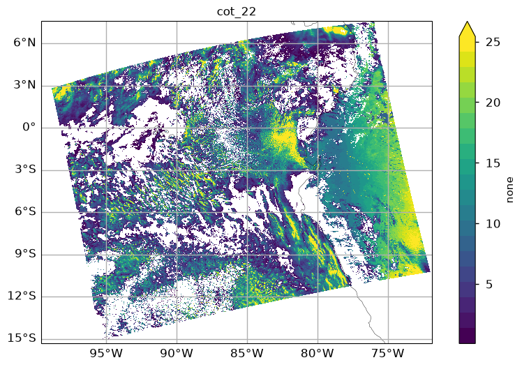
cot_22	none	Cloud Optical Thickness at 670 nm two-channel retrieval using the 1.6 um band and either the 0.65 um, 0.86 um, or 1.2 um band (specified in cld_non_abs_band)
cot_21	none	Cloud Optical Thickness at 670 nm two-channel retrieval using the 1.6 um band and either the 0.65 um, 0.86 um, or 1.2 um band (specified in cld_non_abs_band)
cot_16	none	Cloud Optical Thickness at 670 nm two-channel retrieval using the 1.6 um band and either the 0.65 um, 0.86 um, or 1.2 um band (specified in cld_non_abs_band)
cth_cot		Cloud optical thickness at 760 nm from cloud top height algorithm"
cth_dcot		Estimated 1-sigma uncertainty on retrieved COT at 760 nm from cloud top height algorithm

print_variable_description(dataset, "cer")

	Units	Description
cer_22	micron	Cloud Particle Effective Radius two-channel retrieval using the 2.2 um band and either the 0.65 um, 0.86 um, or 1.2 um band (specified in cld_non_abs_band)
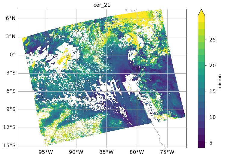
cer_21	micron	Cloud Particle Effective Radius two-channel retrieval using the 2.1 um band and either the 0.65 um, 0.86 um, or 1.2 um band (specified in cld_non_abs_band)
cer_16	micron	Cloud Particle Effective Radius two-channel retrieval using the 1.6 um band and either the 0.65 um, 0.86 um, or 1.2 um band (specified in cld_non_abs_band)

Cloud Phase and Other Properties

Additional variables include cloud phase information and other cloud properties.

print_variable_description(dataset)

	Units	Description
cer_22	micron	Cloud Particle Effective Radius two-channel retrieval using the 2.2 um band and either the 0.65 um, 0.86 um, or 1.2 um band (specified in cld_non_abs_band)
cot_22	none	Cloud Optical Thickness at 670 nm two-channel retrieval using the 1.6 um band and either the 0.65 um, 0.86 um, or 1.2 um band (specified in cld_non_abs_band)
cwp_22	g/m^2	Cloud Column Water Path two-channel retrieval using the 2.2 um band and either the 0.65 um, 0.86 um, or 1.2 um band (specified in cld_non_abs_band)
cer_21	micron	Cloud Particle Effective Radius two-channel retrieval using the 2.1 um band and either the 0.65 um, 0.86 um, or 1.2 um band (specified in cld_non_abs_band)
cot_21	none	Cloud Optical Thickness at 670 nm two-channel retrieval using the 1.6 um band and either the 0.65 um, 0.86 um, or 1.2 um band (specified in cld_non_abs_band)
cwp_21	g/m^2	Cloud Column Water Path two-channel retrieval using the 2.1 um band and either the 0.65 um, 0.86 um, or 1.2 um band (specified in cld_non_abs_band)
cer_16	micron	Cloud Particle Effective Radius two-channel retrieval using the 1.6 um band and either the 0.65 um, 0.86 um, or 1.2 um band (specified in cld_non_abs_band)
cot_16	none	Cloud Optical Thickness at 670 nm two-channel retrieval using the 1.6 um band and either the 0.65 um, 0.86 um, or 1.2 um band (specified in cld_non_abs_band)
cwp_16	g/m^2	Cloud Column Water Path two-channel retrieval using the 1.6 um band and either the 0.65 um, 0.86 um, or 1.2 um band (specified in cld_non_abs_band)
ctp	mbar	Air pressure at the cloud top
ctt	degree K	Air temperature at the cloud top
cth	kilometers	Height at the cloud top
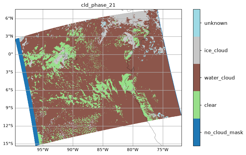
cld_phase_21		Index of the cloud phase derived for the 2100 nm products: 0 - no cloud mask, 1 - clear, 2 - water cloud, 3 - ice cloud, 4 - unknown, assume water cloud
cld_phase_22		Index of the cloud phase derived for the 2200 nm products: 0 - no cloud mask, 1 - clear, 2 - water cloud, 3 - ice cloud, 4 - unknown, assume water cloud
cld_phase_16		Index of the cloud phase derived for the 1600 nm products: 0 - no cloud mask, 1 - clear, 2 - water cloud, 3 - ice cloud, 4 - unknown, assume water cloud
cld_non_abs_band		Non-absorbing band used for 2-channel cloud retrieval: 0 - none, 1 - around 650 nm (for land surface), 2 = around 860 (for water surface), 3 - around 1200 (ice/snow surface)
cth_phase	none	Cloud phase determined by cloud top height algorithm: 0 - water, 1 - ice
cth_cot		Cloud optical thickness at 760 nm from cloud top height algorithm"
cth_cost		Retrieval cost at solution for best-fit cloud optical model
cth_iter		Number of iterations to convergence for best-fit cloud optical model
cth_alb		Best surface albedo made by cloud top height algorithm
cth_dcot		Estimated 1-sigma uncertainty on retrieved COT at 760 nm from cloud top height algorithm
cth_dcth	kilometers	Estimated 1sigma uncertainty on retrieved CTH for best-fit cloud optical model, km
cth_dctp	kilometers	Estimated 1sigma uncertainty on retrieved CTP for best-fit cloud optical model, mb
cth_dctt	degree K	Estimated 1sigma uncertainty on retrieved CTT for best-fit cloud optical model, K
cth_dalb		Estimated 1sigma uncertainty on retrieved surface albedo for best-fit cloud optical model
ice_cloud		Ice cloud fraction for this pixel: 0 - none, 1 - cloud
water_cloud		Water cloud fraction for this pixel: 0 - none, 1 - cloud
l2_flags		Level-2 Processing Flags

4. Visualizing Variables

To visualize the L2 variables, we plot them on cartopy GeoAxes dressed up with our geo_axis_tags function with the color range limited by our extremes_removed_limits function.

help(geo_axis_tags)

Help on function geo_axis_tags in module __main__:

geo_axis_tags(ax, crs=None)
    Add coastlines and labeled latitude/longitude gridlines to a Cartopy axis.

    Parameters
    ----------
    ax : cartopy.mpl.geoaxes.GeoAxes
        Axes object on which to draw the gridlines and coastlines.
    crs : cartopy.crs.CRS, optional
        Coordinate reference system used for the gridlines.
        Default is a Plate Carrée projection with central longitude = 0.

help(extremes_removed_limits)

Help on function extremes_removed_limits in module __main__:

extremes_removed_limits(array)
    Return suggested min and max axis limits based on the interquartile range (IQR) rule.

    Parameters
    ----------
    array : array-like
        Input numeric array.

    Returns
    -------
    tuple
        Suggested min and max for axis limits in plots

Cloud Effective Radius

Visualize the cloud effective radius retrieved from OCI observations. The colorbar limits are adjusted based on the range of observed effective radii, excluding extreme values.

fig, ax = plt.subplots(figsize=(10, 6), subplot_kw={"projection": projection})
var = "cer_21"
array = dataset[var]
vmin, vmax = extremes_removed_limits(array)
cmap = plt.get_cmap("viridis", 20)
img = array.plot.pcolormesh(
    x="longitude",
    y="latitude",
    cmap=cmap,
    vmin=vmin,
    vmax=vmax,
)
img.colorbar.set_label(array.attrs.get("units", ""))
ax.set_title(var, size=12)
geo_axis_tags(ax, projection)
plt.show()

Cloud Optical Thickness

Cloud optical thickness provides information about the opacity of clouds to solar radiation.

fig, ax = plt.subplots(figsize=(10, 6), subplot_kw={"projection": projection})
var = "cot_22"
array = dataset[var]
vmin, vmax = extremes_removed_limits(array)
cmap = plt.get_cmap("viridis", 20)
img = array.plot.pcolormesh(
    x="longitude",
    y="latitude",
    cmap=cmap,
    vmin=vmin,
    vmax=vmax,
)
img.colorbar.set_label(array.attrs.get("units", ""))
ax.set_title(var, size=12)
geo_axis_tags(ax, projection)
plt.show()

Cloud Phase

Cloud phase classification distinguishes between liquid and ice clouds. These variables are discrete, also known as categorical, which we visualize with our plot_cloud_phase function.

help(plot_cloud_phase)

Help on function plot_cloud_phase in module __main__:

plot_cloud_phase(dataset, name, ax)
    Plot a map of cloud phase, a categorical variable, on a cartopy GeoAxes

    Parameters
    ----------
    dataset: xarray.Dataset
        The granule with cloud phase variables
    name: str
        The name of a variable with categorical values
    ax : cartopy.mpl.geoaxes.GeoAxes
        Axes object on which to draw the gridlines and coastlines.

fig, ax = plt.subplots(figsize=(10, 6), subplot_kw={"projection": projection})
plot_cloud_phase(dataset, "cld_phase_21", ax)
plt.show()

5. Reference

• Platnick, S., Meyer, K., King, M. D., Wind, G., Amarasinghe, N., Marchant, B., Arnold, G. T., Zhang, Z., Hubanks, P. A., Ridgway, B., & Riedi, J. (2017). The MODIS Cloud Optical and Microphysical Products: Collection 6 Updates and Examples From Terra and Aqua. IEEE Transactions on Geoscience and Remote Sensing, 55(1), 502–525. https://doi.org/10.1109/TGRS.2016.2610522

• Sayer, A. M., Cairns, B., Knobelspiesse, K. D., Lelli, L., Rajapakshe, C., Giangrande, S. E., Thomas, G. E., and Zhang, D.: Evaluation of cloud height, optical thickness, and phase retrievals from the CHROMA algorithm applied to Sentinel-3 OLCI data, Atmos. Meas. Tech., 18, 6681–6703, https://doi.org/10.5194/amt-18-6681-2025, 2025.

You have completed the notebook on OCI cloud products. May we suggest studying the notebook on HARP2 cloud products?