Explore Level-2 Ocean Color Data from the Moderate Resolution Imaging Spectroradiometer (MODIS)

Author(s): Guoqing Wang (NASA, GSFC), Ian Carroll (NASA, UMBC), Eli Holmes (NOAA), Anna Windle (NASA, GSFC)

Last updated: August 3, 2025

An Earthdata Login account is required to access data from the NASA Earthdata system, including NASA ocean color data.

Summary

This tutorial demonstrates accessing and analyzing NASA ocean color data using Python from the NASA Ocean Biology Distributed Active Archive Center (OB.DAAC) archives. Currently, there are several ways to find and access ocean color data:

1. NASA’s Earthdata Search

2. NASA’s CMR API

3. OB.DAAC OPENDAP

4. OB.DAAC File Search

In this tutorial, we will focus on using earthaccess Python module to access MODIS Aqua ocean color data through NASA’s Common Metadata Repository (CMR), a metadata system that catalogs Earth Science data and associated metadata records. The level 2 dataset of MODIS Aqua is one of the most popular datasets of OB.DAAC. Here we will use MODIS Aqua L2 Chlorophyll a data of the Chesapeake Bay as an example. The standard NASA ocean color Chlorophyll a algorithm is described in the Algorithm Theoretical Basis Document (ATBD).

Learning Objectives

At the end of this notebok you will know:

• How to find OB.DAAC ocean color data

• How to download files using earthaccess

• How to create a plot using xarray

1. Setup

We begin by importing all of the packages used in this notebook. If you have created an environment following the guidance provided with this tutorial, then the imports will be successful.

import cartopy
import earthaccess
import matplotlib.pyplot as plt
import numpy as np
import xarray as xr
from IPython.display import JSON

2. NASA Earthdata Authentication

Next, we authenticate using our Earthdata Login credentials. Authentication is not needed to search publicaly available collections in Earthdata, but is always needed to access data. We can use the login method from the earthaccess package. This will create an authenticated session when we provide a valid Earthdata Login username and password. The earthaccess package will search for credentials defined by environmental variables or within a .netrc file saved in the home directory. If credentials are not found, an interactive prompt will allow you to input credentials.

The persist=True argument ensures any discovered credentials are stored in a .netrc file, so the argument is not necessary (but it's also harmless) for subsequent calls to earthaccess.login.

auth = earthaccess.login(persist=True)

3. Search for Data

The MODIS instrument, on board the Aqua satellite, collects ocean color data, processed from Level-1 through Level-4 and distributed by the OB.DAAC. In this example, we will use the standard Chlorophyll a data from Level-2 (L2) ocean color files. To find data we will use the earthaccess Python library to search on NASA’s CMR API.

NASA data collections, i.e. a series of related granules, are discoverable with earthaccess.search_datasets. Various search parameters can be used to search collections and granules using metadata attributes. See more details here. Below, CMR Catalog are queried to find collections with “L2 ocean color” keyword in them, with the MODIS instrument. The returned response can be used to retrieve the ShortName and concept-id for each dataset.

results = earthaccess.search_datasets(
    keyword="L2 ocean color",
    instrument="MODIS",
)

Each result has a summary method with information such as the collection’s short-name.

set((i.summary()["short-name"] for i in results))

{'MODISA_L2_IOP',
 'MODISA_L2_IOP_NRT',
 'MODISA_L2_OC',
 'MODISA_L2_OC_NRT',
 'MODISA_L2_SST',
 'MODISA_L2_SST4',
 'MODISA_L2_SST4_NRT',
 'MODISA_L2_SST_NRT',
 'MODIST_L2_IOP',
 'MODIST_L2_IOP_NRT',
 'MODIST_L2_OC',
 'MODIST_L2_OC_NRT',
 'MODIST_L2_SST',
 'MODIST_L2_SST4',
 'MODIST_L2_SST4_NRT',
 'MODIST_L2_SST_NRT',
 'NASA_MODIS_RAPID_RESPONSE',
 'WEBCOAST_US_MOD_SST-CHL',
 'gov.noaa.nodc:CoastWatch-OC-Frontal'}

We are interested in the MODISA_L2_OC dataset.

We can use spatial and temporal arguments to search for granules covering Chesapeake Bay during the time frame of Oct 15 - 23, 2020. We can also add the cloud_cover parameter to filter out granules with too much cloud coverage. cloud_cover = (0, 50) # max 50% of cloud coverage

tspan = ("2020-10-15", "2020-10-23")
bbox = (-76.75, 36.97, -75.74, 39.01)
cc = (0, 50)
results = earthaccess.search_data(
    short_name="MODISA_L2_OC",
    temporal=tspan,
    bounding_box=bbox,
    cloud_cover=cc,
)

Now we can print some info about these granules using the built-in methods. We can see how each result prefers to display itself.

results[0]

Data: AQUA_MODIS.20201016T174500.L2.OC.nc

Size: 69.73 MB

Cloud Hosted: True

Or we could use the data_links and size methods provided on each result.

data_links = [{"links": i.data_links(), "size (MB):": i.size()} for i in results]
JSON(data_links, expanded=True)

<IPython.core.display.JSON object>

Or we can interactively inspect all the fields underlying all results.

JSON(results)

<IPython.core.display.JSON object>

4. Download Data

Since the data are not hosted in the Earthdata Cloud (see output from results[0] above), we need to download files. This will download the data in a folder called “data” in your working directory.

paths = earthaccess.download(results, local_path="L2")

5. Plot Data

Step-by-step, we’ll build a nice map showing the log-transformed chlorophyll a estimate for the first granule we downloaded. The first step is to open some of the “groups” present within the NetCDF files to begin preparing a variable to plot.

prod = xr.open_dataset(paths[0])
obs = xr.open_dataset(paths[0], group="geophysical_data")
nav = xr.open_dataset(paths[0], group="navigation_data")

The “navigation_data” group has geospatial coordinates that we merge into the “geophysical_data” group, which has the “chlor_a” product.

nav = nav.set_coords(("longitude", "latitude")).rename(
    {"pixel_control_points": "pixels_per_line"}
)
dataset = xr.merge((prod, obs, nav.coords))

Now, we can pull out and fine-tune the “chlor_a” variable for visualization.

array = np.log10(dataset["chlor_a"])
array.attrs.update(
    {
        "units": f'log10({dataset["chlor_a"].attrs["units"]})',
    }
)

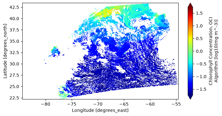
The plot method from XArray’s plotting API is an easy way to take an xr.Dataset or xr.DataArray to a matplotlib figure.

plot = array.plot(x="longitude", y="latitude", aspect=2, size=4, cmap="jet", robust=True)

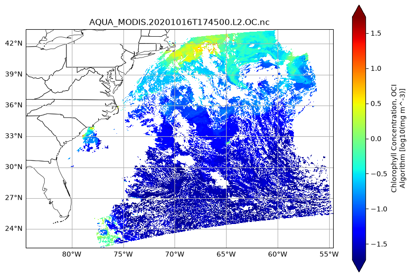
We can enrich the visualiation using matplotlib and cartopy. The coordinates are latitude and longitude, so if we add the “Plate Carree” coordinate reference system (CRS) to our axes, we will get an improved map.

fig, ax = plt.subplots(figsize=(10, 7), subplot_kw={"projection": cartopy.crs.PlateCarree()})
plot = array.plot(x="longitude", y="latitude", cmap="jet", robust=True, ax=ax)
ax.gridlines(draw_labels={"bottom": "x", "left": "y"})
ax.add_feature(cartopy.feature.STATES, linewidth=0.5)
ax.set_title(dataset.attrs["product_name"], loc="center")
plt.show()

You have completed the notebook on Aqua/MODIS L2 data exploration.