

Subsetting PACE OCI data#
Authors: Anna Windle (NASA, SSAI), Carina Poulin (NASA, SSAI), Ian Carroll (NASA, UMBC)
Last Updated: July 7, 2026
The following notebooks are prerequisites for this tutorial.
Learn with OCI: Data Access
An Earthdata Login account is required to access data from the NASA Earthdata system, including NASA ocean color data.
Summary#
This tutorial demonstrates how to subset PACE OCI L2 and L3M data. L2 data is subsetted here using harmony-py, while L3M data is subsetted using xarray.
Harmony is a web service that allows you to customize many NASA datasets, including the ability to subset, reproject, and reformat files. Data can be subsetted for a geographic region, a temporal range and by variable. In some cases, data can be “reprojected” from its native coordinate reference system (CRS) to the coordinate reference system relevant to your analysis. Data can also be reformatted from its native file format to a format that is more relevant for your application. These services are collectively called transformation services. However, not all services and transformations are available for all datasets. You will learn how to discover which services are available for a given dataset.
Harmony services can be used in multiple ways:
through a graphical user interface (GUI) while downloading applicable granules from Earthdata Search,
by direct requests to Harmony’s RESTful API,
through SeaDAS ≥ 11.0.0,
or, as in this tutorial, using the
harmony-pyPython package.
The Python package handles NASA Earthdata Login (EDL) authentication and optionally integrates with the CMR Python Wrapper by accepting collection results as a request parameter. It’s convenient for scientists who wish to use Harmony from Jupyter notebooks.
After this tutorial, you can dive deeper into harmony-py on ReadTheDocs.
This tutorial demonstrates how to subset and reformat PACE OCI data from the NASA Earthdata Cloud using harmony-py. It is modelled off of tutorials developed by NSIDC and NASA-Openscapes.
Learning Objectives#
At the end of this notebook you will know how to:
Use the
harmony-pyPython library to spatially and temporally subset PACE OCI Level-2 dataDownload the subsetted data to your local directory
Stream the subsetted data
Open and plot subsetted L2 PACE OCI data
Open and subset PACE OCI Level-3 mapped data using
xarray
1. Setup#
Begin by importing all of the packages used in this notebook.
from datetime import datetime
from pathlib import Path

import earthaccess
import matplotlib.pyplot as plt
import numpy as np
import rasterio
import xarray as xr
import rioxarray
from harmony import (
    BBox,
    CapabilitiesRequest,
    Client,
    Collection,
    JobsRequest,
    LinkType,
    Request,
)
from rasterio.enums import Resampling
2. Earthdata authentication and Harmony client initalization#
The earthaccess package lets us easily authenticate with NASA’s Earthdata Login (EDL) and pass an EDL token to Harmony.
auth = earthaccess.login()
harmony_client = Client(token=earthaccess.get_edl_token())
3. Discover subsetting capabilities for Level-2 PACE OCI data#
Define which data set you’d like to access using either the dataset short_name or its collection concept_id. For this example, we’ll use PACE OCI Level-2 Regional Ocean Biogeochemical Properties Data (PACE_OCI_L2_BGC).
capabilities_request = CapabilitiesRequest(short_name="PACE_OCI_L2_BGC")
capabilities = harmony_client.submit(capabilities_request)
capabilities
{'conceptId': 'C4124887072-OB_CLOUD',
 'shortName': 'PACE_OCI_L2_BGC',
 'variableSubset': True,
 'bboxSubset': True,
 'shapeSubset': True,
 'temporalSubset': True,
 'concatenate': False,
 'reproject': False,
 'outputFormats': ['application/netcdf'],
 'services': [{'name': 'podaac/l2-subsetter',
   'href': 'https://cmr.earthdata.nasa.gov/search/concepts/S1962070864-POCLOUD',
   'capabilities': {'subsetting': {'temporal': True,
     'bbox': True,
     'variable': True,
     'shape': True,
     'dimension': True},
    'output_formats': ['application/netcdf']}}],
 'variables': [{'name': 'geophysical_data/carbon_phyto',
   'href': 'https://cmr.earthdata.nasa.gov/search/concepts/V4198030748-OB_CLOUD'},
  {'name': 'geophysical_data/carbon_phyto_unc',
   'href': 'https://cmr.earthdata.nasa.gov/search/concepts/V4198030761-OB_CLOUD'},
  {'name': 'geophysical_data/chlor_a',
   'href': 'https://cmr.earthdata.nasa.gov/search/concepts/V4198030774-OB_CLOUD'},
  {'name': 'geophysical_data/chlor_a_unc',
   'href': 'https://cmr.earthdata.nasa.gov/search/concepts/V4198030781-OB_CLOUD'},
  {'name': 'geophysical_data/l2_flags',
   'href': 'https://cmr.earthdata.nasa.gov/search/concepts/V4241067558-OB_CLOUD'},
  {'name': 'geophysical_data/pic',
   'href': 'https://cmr.earthdata.nasa.gov/search/concepts/V4198030803-OB_CLOUD'},
  {'name': 'geophysical_data/poc',
   'href': 'https://cmr.earthdata.nasa.gov/search/concepts/V4198030812-OB_CLOUD'}],
 'capabilitiesVersion': '2'}
You can see here under ['services'] that this dataset can be subsetted using the 'podacc/l2-subsetter'
4. Build and submit a request#
The Harmony service is based around user-submitted jobs. Using the service is a two-step process of (1) creating a specific type of request, and (2) passing the request to the harmony_client in exchange for some response from Harmony.
One type of request, the JobsRequest, let’s you check for any previously submitted jobs. You can filter these jobs using labels, which we will learn how to apply below.
First step, create a request:
request = JobsRequest(labels=["help-hub-tutorial"])
Second, get a response from your request submission:
response = harmony_client.submit(request)
response["count"]
1
For your first time through this tutorial, you shouldn’t see any existing jobs. If you’ve already submitted a job with this label (e.g. because you are re-running this tutorial), then the response includes information about that existing job.
Let’s continue to build a request for the subsetting job we want the service to run. Using the “labels” keyword tags jobs so that we can easily find and re-use results from this job later.
request = Request(
    collection=Collection(id="PACE_OCI_L2_BGC"),
    spatial=BBox(-76.75, 36.97, -75.74, 39.01),
    temporal={"start": datetime(2025, 7, 1), "stop": datetime(2025, 8, 1)},
    variables=["geophysical_data/chlor_a", "geophysical_data/l2_flags"],
    pixel_subset=True,
    labels=request.labels,
)
Depending on whether we got a non-zero count from the JobsRequest, we can either submit the subsetting request or dig into the job info we retrieved. Either way, we come up with a job_id that uniquely identifies the subsetting job.
if response["count"]:
    job_id = response["jobs"][0]["jobID"]
else:
    job_id = harmony_client.submit(request)
job_id
'12fce294-ebfa-4c00-82fa-0beb552ba0f9'
The job_id can be used to check on the details of your job progress. If you are logged into Earthdata, you can see your jobs here: https://harmony.earthdata.nasa.gov/workflow-ui
or look at your process by running this line:
harmony_client.wait_for_processing(job_id, show_progress=True)
 [ Processing:   0% ] |                                                   | [/]
 [ Processing: 100% ] |###################################################| [|]
Note: Requesting a job can take a variable amount of time. In our experience, running this particular job has ranged from 2 to 24 minutes.
job_summary = harmony_client.result_json(job_id)
print("Number of granules:", job_summary["numInputGranules"])
print("Original Data Size:", job_summary["originalDataSize"])
print("Output Data Size:", job_summary["outputDataSize"])
print("Data Size % Change:", job_summary["dataSizePercentChange"])
Number of granules: 44
Original Data Size: 759.11 MiB
Output Data Size: 5.94 MiB
Data Size % Change: 99.22% reduction
If you want to access a specific job that has already run, you can simply assign a known id to job_id and continue below.
Results are kept for 30 days in the Harmony S3 bucket.
5. Access the subsetted data#
The subsetted files can be accessed by downloading the files to a local machine, or by streaming the data. We will use both access methods in the examples below.
Download a single file#
The download method takes a url to a single subsetted file. There are two optional arguments; directory used to specify an existing folder for storing data (defaults to the current directory), and overwrite which defaults to False to avoid downloading the same file twice. If you need to download the file again, then set overwrite=True.
Let’s download the first granule:
url = list(harmony_client.result_urls(job_id))[0]
filepath = harmony_client.download(url).result()
257336916_PACE_OCI.20250701T181813.L2.OC_BGC.V3_2_subsetted.nc
You should see this file saved in your local directory.
You can also make a new folder in your local directory to save the subsetted data. Here, we are naming it “subsetted_data”:
subsetted_data = Path("subsetted_data")
subsetted_data.mkdir(exist_ok=True)

filepath = harmony_client.download(url, directory=subsetted_data).result()
subsetted_data/257336916_PACE_OCI.20250701T181813.L2.OC_BGC.V3_2_subsetted.nc
Download all files#
The download_all method can use the job_id or the result_json, which contains result URLs.
As with download, the download directory path on the local machine can be specified with the directory keyword. To save downloading the same file, the overwrite keyword can be set to False.
The paths fo the files are returned as a list.
futures = harmony_client.download_all(job_id, directory=subsetted_data)
filelist = [f.result() for f in futures]
subsetted_data/257336916_PACE_OCI.20250701T181813.L2.OC_BGC.V3_2_subsetted.nc
subsetted_data/257336915_PACE_OCI.20250701T163952.L2.OC_BGC.V3_2_subsetted.nc
subsetted_data/257336917_PACE_OCI.20250702T171504.L2.OC_BGC.V3_2_subsetted.nc
subsetted_data/257336918_PACE_OCI.20250703T175015.L2.OC_BGC.V3_2_subsetted.nc
subsetted_data/257336919_PACE_OCI.20250704T164706.L2.OC_BGC.V3_2_subsetted.nc
subsetted_data/257336920_PACE_OCI.20250704T182527.L2.OC_BGC.V3_2_subsetted.nc
subsetted_data/257336921_PACE_OCI.20250705T172218.L2.OC_BGC.V3_2_subsetted.nc
subsetted_data/257336922_PACE_OCI.20250706T175729.L2.OC_BGC.V3_2_subsetted.nc
subsetted_data/257336923_PACE_OCI.20250707T165419.L2.OC_BGC.V3_2_subsetted.nc
subsetted_data/257336924_PACE_OCI.20250707T183240.L2.OC_BGC.V3_2_subsetted.nc
subsetted_data/257336925_PACE_OCI.20250708T172930.L2.OC_BGC.V3_2_subsetted.nc
subsetted_data/257336926_PACE_OCI.20250709T162620.L2.OC_BGC.V3_2_subsetted.nc
subsetted_data/257336927_PACE_OCI.20250709T180441.L2.OC_BGC.V3_2_subsetted.nc
subsetted_data/257336928_PACE_OCI.20250710T170131.L2.OC_BGC.V3_2_subsetted.nc
subsetted_data/257336929_PACE_OCI.20250710T183952.L2.OC_BGC.V3_2_subsetted.nc
subsetted_data/257336930_PACE_OCI.20250711T173641.L2.OC_BGC.V3_2_subsetted.nc
subsetted_data/257336931_PACE_OCI.20250712T163331.L2.OC_BGC.V3_2_subsetted.nc
subsetted_data/257336933_PACE_OCI.20250713T170841.L2.OC_BGC.V3_2_subsetted.nc
subsetted_data/257336932_PACE_OCI.20250712T181152.L2.OC_BGC.V3_2_subsetted.nc
subsetted_data/257336934_PACE_OCI.20250714T174351.L2.OC_BGC.V3_2_subsetted.nc
subsetted_data/257336935_PACE_OCI.20250715T164041.L2.OC_BGC.V3_2_subsetted.nc
subsetted_data/257336936_PACE_OCI.20250715T181901.L2.OC_BGC.V3_2_subsetted.nc
subsetted_data/257336937_PACE_OCI.20250716T171550.L2.OC_BGC.V3_2_subsetted.nc
subsetted_data/257336938_PACE_OCI.20250717T175100.L2.OC_BGC.V3_2_subsetted.nc
subsetted_data/257336939_PACE_OCI.20250718T164749.L2.OC_BGC.V3_2_subsetted.nc
subsetted_data/257336940_PACE_OCI.20250718T182610.L2.OC_BGC.V3_2_subsetted.nc
subsetted_data/257336942_PACE_OCI.20250720T175808.L2.OC_BGC.V3_2_subsetted.nc
subsetted_data/257336941_PACE_OCI.20250719T172258.L2.OC_BGC.V3_2_subsetted.nc
subsetted_data/257336943_PACE_OCI.20250721T165456.L2.OC_BGC.V3_2_subsetted.nc
subsetted_data/257336944_PACE_OCI.20250721T183317.L2.OC_BGC.V3_2_subsetted.nc
subsetted_data/257336945_PACE_OCI.20250722T173005.L2.OC_BGC.V3_2_subsetted.nc
subsetted_data/257336946_PACE_OCI.20250723T162654.L2.OC_BGC.V3_2_subsetted.nc
subsetted_data/257336947_PACE_OCI.20250723T180514.L2.OC_BGC.V3_2_subsetted.nc
subsetted_data/257336948_PACE_OCI.20250724T170203.L2.OC_BGC.V3_2_subsetted.nc
subsetted_data/257336950_PACE_OCI.20250725T173711.L2.OC_BGC.V3_2_subsetted.nc
subsetted_data/257336951_PACE_OCI.20250726T163400.L2.OC_BGC.V3_2_subsetted.nc
subsetted_data/257336952_PACE_OCI.20250726T181220.L2.OC_BGC.V3_2_subsetted.nc
subsetted_data/257336954_PACE_OCI.20250728T174415.L2.OC_BGC.V3_2_subsetted.nc
subsetted_data/257336955_PACE_OCI.20250729T164102.L2.OC_BGC.V3_2_subsetted.nc
subsetted_data/257336953_PACE_OCI.20250727T170908.L2.OC_BGC.V3_2_subsetted.nc
subsetted_data/257336956_PACE_OCI.20250729T181923.L2.OC_BGC.V3_2_subsetted.nc
subsetted_data/257336957_PACE_OCI.20250730T171610.L2.OC_BGC.V3_2_subsetted.nc
subsetted_data/257336958_PACE_OCI.20250731T175118.L2.OC_BGC.V3_2_subsetted.nc
len(filelist)
43
You can now open the files using xarray.
dt = xr.open_datatree(filelist[0])
ds = xr.merge(dt.to_dict().values())
ds = ds.set_coords(("longitude", "latitude"))
ds
<xarray.Dataset> Size: 108kB
Dimensions:    (number_of_lines: 202, pixels_per_line: 33)
Coordinates:
    longitude  (number_of_lines, pixels_per_line) float32 27kB ...
    latitude   (number_of_lines, pixels_per_line) float32 27kB ...
Dimensions without coordinates: number_of_lines, pixels_per_line
Data variables:
    time       (number_of_lines) datetime64[ns] 2kB ...
    chlor_a    (number_of_lines, pixels_per_line) float32 27kB ...
    l2_flags   (number_of_lines, pixels_per_line) int32 27kB ...
Attributes: (12/40)
    title:                             OCI Level-2 Data BGC
    product_name:                      PACE_OCI.20250701T181813.L2.OC_BGC.V3_...
    processing_version:                3.2
    history:                           l2gen par=/data3/sdpsoper/vdc/vpu8/wor...
    instrument:                        OCI
    platform:                          PACE
    ...                                ...
    startDirection:                    Ascending
    endDirection:                      Ascending
    day_night_flag:                    Day
    earth_sun_distance_correction:     0.9674508571624756
    geospatial_bounds:                 POLYGON((-76.72168 36.83092, -77.06343...
history_json: [{"date_time": "2026-07-14T14:20:57.58...There’s no need to keep these files around if you plan to stream the data instead of downloading. You can run this to delete all of the locally downloaded files.
for item in subsetted_data.glob("*.nc*"):
    item.unlink()
Stream the files#
If you are working in the AWS us-west-2 region (the same region as NASA Earthdata Cloud) you can stream the data using direct S3 access.
You must be running this notebook in the AWS us-west-2 region to run the following code cells.
We need to get the url for the data in the S3 bucket. We can do this using result_urls, as we did for download but we set link_type=LinkType.s3 to specify we want the S3 url.
urls = list(harmony_client.result_urls(job_id, link_type=LinkType.s3))
urls
['s3://harmony-prod-staging/public/12fce294-ebfa-4c00-82fa-0beb552ba0f9/257336916/PACE_OCI.20250701T181813.L2.OC_BGC.V3_2_subsetted.nc',
 's3://harmony-prod-staging/public/12fce294-ebfa-4c00-82fa-0beb552ba0f9/257336915/PACE_OCI.20250701T163952.L2.OC_BGC.V3_2_subsetted.nc',
 's3://harmony-prod-staging/public/12fce294-ebfa-4c00-82fa-0beb552ba0f9/257336917/PACE_OCI.20250702T171504.L2.OC_BGC.V3_2_subsetted.nc',
 's3://harmony-prod-staging/public/12fce294-ebfa-4c00-82fa-0beb552ba0f9/257336918/PACE_OCI.20250703T175015.L2.OC_BGC.V3_2_subsetted.nc',
 's3://harmony-prod-staging/public/12fce294-ebfa-4c00-82fa-0beb552ba0f9/257336919/PACE_OCI.20250704T164706.L2.OC_BGC.V3_2_subsetted.nc',
 's3://harmony-prod-staging/public/12fce294-ebfa-4c00-82fa-0beb552ba0f9/257336920/PACE_OCI.20250704T182527.L2.OC_BGC.V3_2_subsetted.nc',
 's3://harmony-prod-staging/public/12fce294-ebfa-4c00-82fa-0beb552ba0f9/257336921/PACE_OCI.20250705T172218.L2.OC_BGC.V3_2_subsetted.nc',
 's3://harmony-prod-staging/public/12fce294-ebfa-4c00-82fa-0beb552ba0f9/257336922/PACE_OCI.20250706T175729.L2.OC_BGC.V3_2_subsetted.nc',
 's3://harmony-prod-staging/public/12fce294-ebfa-4c00-82fa-0beb552ba0f9/257336923/PACE_OCI.20250707T165419.L2.OC_BGC.V3_2_subsetted.nc',
 's3://harmony-prod-staging/public/12fce294-ebfa-4c00-82fa-0beb552ba0f9/257336924/PACE_OCI.20250707T183240.L2.OC_BGC.V3_2_subsetted.nc',
 's3://harmony-prod-staging/public/12fce294-ebfa-4c00-82fa-0beb552ba0f9/257336925/PACE_OCI.20250708T172930.L2.OC_BGC.V3_2_subsetted.nc',
 's3://harmony-prod-staging/public/12fce294-ebfa-4c00-82fa-0beb552ba0f9/257336926/PACE_OCI.20250709T162620.L2.OC_BGC.V3_2_subsetted.nc',
 's3://harmony-prod-staging/public/12fce294-ebfa-4c00-82fa-0beb552ba0f9/257336927/PACE_OCI.20250709T180441.L2.OC_BGC.V3_2_subsetted.nc',
 's3://harmony-prod-staging/public/12fce294-ebfa-4c00-82fa-0beb552ba0f9/257336928/PACE_OCI.20250710T170131.L2.OC_BGC.V3_2_subsetted.nc',
 's3://harmony-prod-staging/public/12fce294-ebfa-4c00-82fa-0beb552ba0f9/257336929/PACE_OCI.20250710T183952.L2.OC_BGC.V3_2_subsetted.nc',
 's3://harmony-prod-staging/public/12fce294-ebfa-4c00-82fa-0beb552ba0f9/257336930/PACE_OCI.20250711T173641.L2.OC_BGC.V3_2_subsetted.nc',
 's3://harmony-prod-staging/public/12fce294-ebfa-4c00-82fa-0beb552ba0f9/257336931/PACE_OCI.20250712T163331.L2.OC_BGC.V3_2_subsetted.nc',
 's3://harmony-prod-staging/public/12fce294-ebfa-4c00-82fa-0beb552ba0f9/257336933/PACE_OCI.20250713T170841.L2.OC_BGC.V3_2_subsetted.nc',
 's3://harmony-prod-staging/public/12fce294-ebfa-4c00-82fa-0beb552ba0f9/257336932/PACE_OCI.20250712T181152.L2.OC_BGC.V3_2_subsetted.nc',
 's3://harmony-prod-staging/public/12fce294-ebfa-4c00-82fa-0beb552ba0f9/257336934/PACE_OCI.20250714T174351.L2.OC_BGC.V3_2_subsetted.nc',
 's3://harmony-prod-staging/public/12fce294-ebfa-4c00-82fa-0beb552ba0f9/257336935/PACE_OCI.20250715T164041.L2.OC_BGC.V3_2_subsetted.nc',
 's3://harmony-prod-staging/public/12fce294-ebfa-4c00-82fa-0beb552ba0f9/257336936/PACE_OCI.20250715T181901.L2.OC_BGC.V3_2_subsetted.nc',
 's3://harmony-prod-staging/public/12fce294-ebfa-4c00-82fa-0beb552ba0f9/257336937/PACE_OCI.20250716T171550.L2.OC_BGC.V3_2_subsetted.nc',
 's3://harmony-prod-staging/public/12fce294-ebfa-4c00-82fa-0beb552ba0f9/257336938/PACE_OCI.20250717T175100.L2.OC_BGC.V3_2_subsetted.nc',
 's3://harmony-prod-staging/public/12fce294-ebfa-4c00-82fa-0beb552ba0f9/257336939/PACE_OCI.20250718T164749.L2.OC_BGC.V3_2_subsetted.nc',
 's3://harmony-prod-staging/public/12fce294-ebfa-4c00-82fa-0beb552ba0f9/257336940/PACE_OCI.20250718T182610.L2.OC_BGC.V3_2_subsetted.nc',
 's3://harmony-prod-staging/public/12fce294-ebfa-4c00-82fa-0beb552ba0f9/257336942/PACE_OCI.20250720T175808.L2.OC_BGC.V3_2_subsetted.nc',
 's3://harmony-prod-staging/public/12fce294-ebfa-4c00-82fa-0beb552ba0f9/257336941/PACE_OCI.20250719T172258.L2.OC_BGC.V3_2_subsetted.nc',
 's3://harmony-prod-staging/public/12fce294-ebfa-4c00-82fa-0beb552ba0f9/257336943/PACE_OCI.20250721T165456.L2.OC_BGC.V3_2_subsetted.nc',
 's3://harmony-prod-staging/public/12fce294-ebfa-4c00-82fa-0beb552ba0f9/257336944/PACE_OCI.20250721T183317.L2.OC_BGC.V3_2_subsetted.nc',
 's3://harmony-prod-staging/public/12fce294-ebfa-4c00-82fa-0beb552ba0f9/257336945/PACE_OCI.20250722T173005.L2.OC_BGC.V3_2_subsetted.nc',
 's3://harmony-prod-staging/public/12fce294-ebfa-4c00-82fa-0beb552ba0f9/257336946/PACE_OCI.20250723T162654.L2.OC_BGC.V3_2_subsetted.nc',
 's3://harmony-prod-staging/public/12fce294-ebfa-4c00-82fa-0beb552ba0f9/257336947/PACE_OCI.20250723T180514.L2.OC_BGC.V3_2_subsetted.nc',
 's3://harmony-prod-staging/public/12fce294-ebfa-4c00-82fa-0beb552ba0f9/257336948/PACE_OCI.20250724T170203.L2.OC_BGC.V3_2_subsetted.nc',
 's3://harmony-prod-staging/public/12fce294-ebfa-4c00-82fa-0beb552ba0f9/257336950/PACE_OCI.20250725T173711.L2.OC_BGC.V3_2_subsetted.nc',
 's3://harmony-prod-staging/public/12fce294-ebfa-4c00-82fa-0beb552ba0f9/257336951/PACE_OCI.20250726T163400.L2.OC_BGC.V3_2_subsetted.nc',
 's3://harmony-prod-staging/public/12fce294-ebfa-4c00-82fa-0beb552ba0f9/257336952/PACE_OCI.20250726T181220.L2.OC_BGC.V3_2_subsetted.nc',
 's3://harmony-prod-staging/public/12fce294-ebfa-4c00-82fa-0beb552ba0f9/257336954/PACE_OCI.20250728T174415.L2.OC_BGC.V3_2_subsetted.nc',
 's3://harmony-prod-staging/public/12fce294-ebfa-4c00-82fa-0beb552ba0f9/257336955/PACE_OCI.20250729T164102.L2.OC_BGC.V3_2_subsetted.nc',
 's3://harmony-prod-staging/public/12fce294-ebfa-4c00-82fa-0beb552ba0f9/257336953/PACE_OCI.20250727T170908.L2.OC_BGC.V3_2_subsetted.nc',
 's3://harmony-prod-staging/public/12fce294-ebfa-4c00-82fa-0beb552ba0f9/257336956/PACE_OCI.20250729T181923.L2.OC_BGC.V3_2_subsetted.nc',
 's3://harmony-prod-staging/public/12fce294-ebfa-4c00-82fa-0beb552ba0f9/257336957/PACE_OCI.20250730T171610.L2.OC_BGC.V3_2_subsetted.nc',
 's3://harmony-prod-staging/public/12fce294-ebfa-4c00-82fa-0beb552ba0f9/257336958/PACE_OCI.20250731T175118.L2.OC_BGC.V3_2_subsetted.nc']
We need AWS credentials to access the S3 bucket with the results. These can be passed when using xr.open_datatree:
kwargs = {
    "engine": "h5netcdf",
    "storage_options": {
        "client_kwargs": harmony_client.aws_credentials(),
    },
}

dt = xr.open_datatree(urls[0], **kwargs)
ds = xr.merge(dt.to_dict().values())
ds = ds.set_coords(("longitude", "latitude"))
ds
<xarray.Dataset> Size: 108kB
Dimensions:    (number_of_lines: 202, pixels_per_line: 33)
Coordinates:
    longitude  (number_of_lines, pixels_per_line) float32 27kB ...
    latitude   (number_of_lines, pixels_per_line) float32 27kB ...
Dimensions without coordinates: number_of_lines, pixels_per_line
Data variables:
    time       (number_of_lines) datetime64[ns] 2kB ...
    chlor_a    (number_of_lines, pixels_per_line) float32 27kB ...
    l2_flags   (number_of_lines, pixels_per_line) int32 27kB ...
Attributes: (12/40)
    title:                             OCI Level-2 Data BGC
    product_name:                      PACE_OCI.20250701T181813.L2.OC_BGC.V3_...
    processing_version:                3.2
    history:                           l2gen par=/data3/sdpsoper/vdc/vpu8/wor...
    instrument:                        OCI
    platform:                          PACE
    ...                                ...
    startDirection:                    Ascending
    endDirection:                      Ascending
    day_night_flag:                    Day
    earth_sun_distance_correction:     0.9674508571624756
    geospatial_bounds:                 POLYGON((-76.72168 36.83092, -77.06343...
history_json: [{"date_time": "2026-07-14T14:20:57.58...6. Plot the subsetted data#
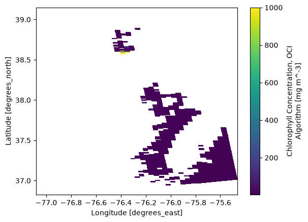
Let’s do a quick plot of chlor_a from the first granule:
plot = ds["chlor_a"].plot(x="longitude", y="latitude")
Now let’s plot multiple subsetted granules:
fig, axes = plt.subplots(2, 5, figsize=(10, 4), constrained_layout=True)
axes = axes.ravel()
da = []

for ax, file in zip(axes, urls[:10]):

    dt = xr.open_datatree(file, **kwargs)
    ds = xr.merge(dt.to_dict().values())
    ds = ds.set_coords(("longitude", "latitude"))

    da.append(ds["chlor_a"])

    date = ds.attrs["time_coverage_start"]
    im = ds["chlor_a"].plot(
        ax=ax,
        x="longitude",
        y="latitude",
        cmap="viridis",
        add_colorbar=False,
        vmin=0,
        vmax=20,
    )
    ax.set_title(date, fontsize=8)

    ax.set_xlabel("")
    ax.set_ylabel("")

fig.colorbar(im, ax=axes, orientation="vertical", shrink=0.8, label="Chl a (mg m-3)")
plt.show()
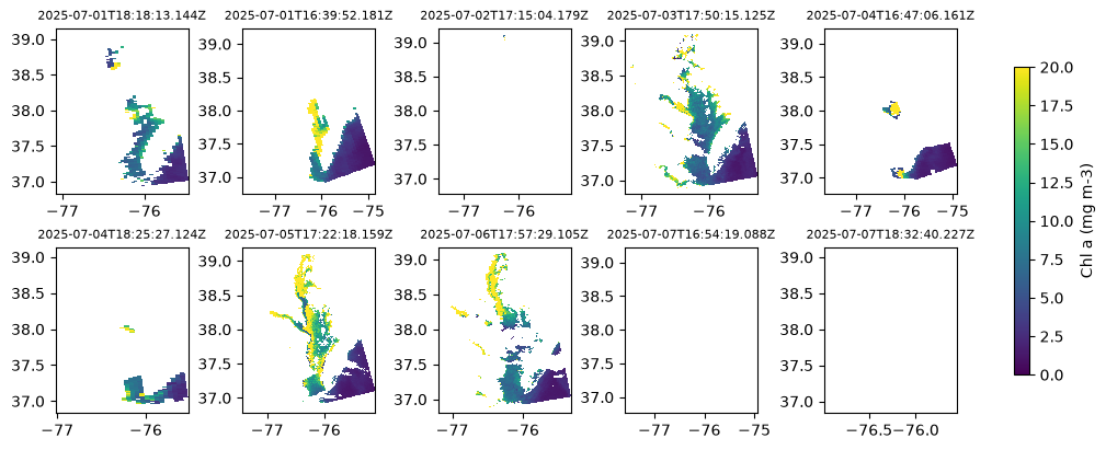
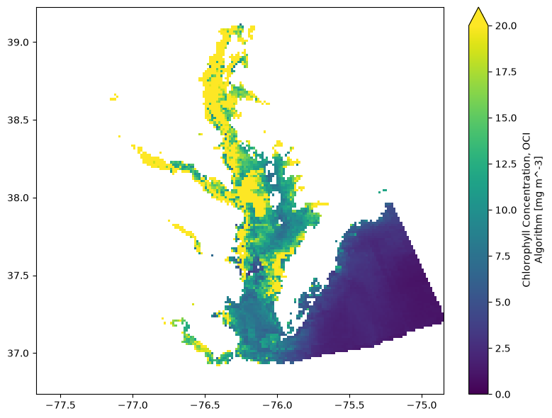
We can also make a L2 composite. However, in order to combine multiple granules into a common spatial framework we need to project the data onto a defined grid with a given reslution. We will use code presented in the Projecting PACE Data onto a Predefined Grid tutorial.
def grid_data(src, resolution, dst_crs="epsg:4326", resampling=Resampling.nearest):
    """
    Reproject a L2 dataset to match an input grid. Makes sure 3D variables are
        in (Z, Y, X) dimension order, and all variables have spatial dims/crs
        assigned.
    Args:
        src - an xarray dataset or dataarray to reproject
        resolution - resolution of the output grid, in dst_crs units
        dst_crs - CRS of the output data
        resampling - resampling method (see rasterio.enums)
    Returns:
        dst - projected xr dataset
    """
    if (len(list(src.dims)) == 3) and (list(src.dims)[0] != "wavelength"):
        src = src.transpose("wavelength", ...)
    src = src.rio.set_spatial_dims("pixels_per_line", "number_of_lines")
    src = src.rio.write_crs("epsg:4326")

    # Calculating the default affine transform
    defaults = rasterio.warp.calculate_default_transform(
        src.rio.crs,
        dst_crs,
        src.rio.width,
        src.rio.height,
        left=src.attrs["geospatial_lon_min"],
        bottom=src.attrs["geospatial_lat_min"],
        right=src.attrs["geospatial_lon_max"],
        top=src.attrs["geospatial_lat_max"],
    )
    # Aligning that transform to our desired resolution
    transform, width, height = rasterio.warp.aligned_target(*defaults, resolution)

    dst = src.rio.reproject(
        dst_crs=dst_crs,
        shape=(height, width),
        transform=transform,
        src_geoloc_array=(
            src["longitude"],
            src["latitude"],
        ),
        nodata=np.nan,
        resample=resampling,
    )
    dst["x"] = dst["x"].round(9)
    dst["y"] = dst["y"].round(9)

    return dst.rename({"x":"longitude", "y":"latitude"})
Now, we can make a 10-day Chl a composite. The l2_flags variable cannot be gridded using this function; if you need to use the l2_flags to mask out additional data, you can do that on the subetted granules before gridding.
gridded_list = []
resolution = (0.015, 0.015)

for file in urls[:10]:

    dt = xr.open_datatree(file, **kwargs)
    ds = xr.merge(dt.to_dict().values())
    ds = ds.set_coords(("longitude", "latitude"))
    ds = ds.drop_vars("l2_flags")

    ds_gridded = grid_data(ds, resolution)

    gridded_list.append(ds_gridded.chlor_a)

stack = xr.concat(gridded_list, dim="scene")

chlor_a_mean = stack.mean(dim="scene", skipna=True)
fig, ax = plt.subplots(figsize=(8, 6))

chlor_a_mean.plot(
    ax=ax,
    cmap="viridis",
    vmin=0,
    vmax=20
)

ax.set_xlabel("")
ax.set_ylabel("")
ax.set_title("")

plt.tight_layout()
plt.show()
7. Subsetting L3M data#
Currently, harmony-py does not support spatial subsetting for PACE OCI L3M products. You can verify this by submitting a Harmony request and inspecting the available services, where the subset capabilities are listed as False.
capabilities_request = CapabilitiesRequest(short_name="PACE_OCI_L3M_BGC")
capabilities = harmony_client.submit(capabilities_request)
capabilities
{'conceptId': 'C4184125847-OB_CLOUD',
 'shortName': 'PACE_OCI_L3M_BGC',
 'variableSubset': False,
 'bboxSubset': False,
 'shapeSubset': False,
 'temporalSubset': False,
 'concatenate': False,
 'reproject': False,
 'outputFormats': [],
 'services': [],
 'variables': [{'name': 'carbon_phyto',
   'href': 'https://cmr.earthdata.nasa.gov/search/concepts/V4200415254-OB_CLOUD'},
  {'name': 'chlor_a',
   'href': 'https://cmr.earthdata.nasa.gov/search/concepts/V4200415263-OB_CLOUD'},
  {'name': 'pic',
   'href': 'https://cmr.earthdata.nasa.gov/search/concepts/V4200415267-OB_CLOUD'},
  {'name': 'poc',
   'href': 'https://cmr.earthdata.nasa.gov/search/concepts/V4200415274-OB_CLOUD'}],
 'capabilitiesVersion': '2'}
Because spatial subsetting is not currently supported for PACE OCI L3M products through Harmony, we will instead use xarray to subset the data locally. Since L3M products are already mapped to a regular spatial grid, this approach is both straightforward and computationally efficient.
Let’s begin by opening a monthly (MO) PACE_OCI_L3M_BGC composite at 4 km spatial resolution using earthaccess:
results = earthaccess.search_data(
    short_name="PACE_OCI_L3M_BGC",
    temporal=("2025-07", "2025-07"),
    granule_name="*.MO.*.4km.*",
)
paths = earthaccess.open(results)
ds = xr.open_dataset(paths[0])
ds
<xarray.Dataset> Size: 597MB
Dimensions:       (lat: 4320, lon: 8640)
Coordinates:
  * lat           (lat) float32 17kB 89.98 89.94 89.9 ... -89.9 -89.94 -89.98
  * lon           (lon) float32 35kB -180.0 -179.9 -179.9 ... 179.9 179.9 180.0
Data variables:
    poc           (lat, lon) float32 149MB ...
    pic           (lat, lon) float32 149MB ...
    chlor_a       (lat, lon) float32 149MB ...
    carbon_phyto  (lat, lon) float32 149MB ...
Attributes: (12/55)
    product_name:                      PACE_OCI.20250701_20250731.L3m.MO.BGC....
    instrument:                        OCI
    title:                             OCI Level-3 Standard Mapped Image
    project:                           Ocean Biology Processing Group (NASA/G...
    platform:                          PACE
    source:                            satellite observations from OCI-PACE
    ...                                ...
    keywords:                          Earth Science > Oceans > Ocean Chemist...
    id:                                L3/PACE_OCI.20250701_20250731.L3m.MO.B...
    history:                           /sdps/sdpsoper/Science/OCSSW/V2026.2/b...
    processing_version:                3.2
    identifier_product_doi_authority:  https://dx.doi.org
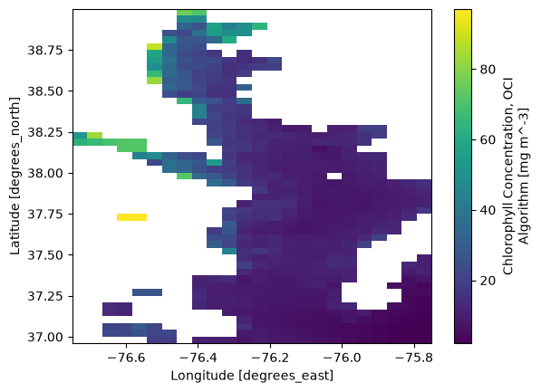
identifier_product_doi: 10.5067/PACE/OCI/L3M/OC_BGC/3.2Now we are going to subset in two ways, first, by selecting a variable with .sel, and secondly by selecting a spatial subset with slice. We can do this all in one line:
ds_sub = ds["chlor_a"].sel({"lat": slice(39.01, 36.97), "lon": slice(-76.75, -75.74)})
plot = ds_sub.plot.imshow()
If we now save this sliced dataset to a netCDF file, we have effectively “downloaded” a subsetted dataset:
subsetted_data = Path("./subsetted_data")
subsetted_data.mkdir(exist_ok=True)
path = subsetted_data / ds.attrs["product_name"]
path = path.with_suffix(".subsetted.nc")
print(path)
subsetted_data/PACE_OCI.20250701_20250731.L3m.MO.BGC.V3_2.4km.subsetted.nc
ds_sub.to_netcdf(path)
You should now see this file in your “subsetted_data” folder. Let’s compare the size to the original L3M file:
og_size = results[0].size()
sub_size = path.stat().st_size / 2**20
print(f"Original Data Size: {og_size:.2f} MB")
print(f"Output Data Size: {sub_size:.2f} MB")
print(f"Data Size % Change: {100 * (1 - sub_size / og_size):.2f} % reduction")
Original Data Size: 134.16 MB
Output Data Size: 0.02 MB
Data Size % Change: 99.99 % reduction
You have completed the notebook on Subsetting PACE OCI data!