Explore Level-3 Ocean Color Data from the Moderate Resolution Imaging Spectroradiometer (MODIS)

Explore Level-3 Ocean Color Data from the Moderate Resolution Imaging Spectroradiometer (MODIS)#

Author(s): Guoqing Wang (NASA, GSFC), Ian Carroll (NASA, UMBC), Eli Holmes (NOAA)

Last updated: August 3, 2025

The following notebooks are prerequisites for this tutorial.

Learn with MODIS: Explore Level-2 Ocean Color Data

An Earthdata Login account is required to access data from the NASA Earthdata system, including NASA ocean color data.

Summary#

This tutorial demonstrates accessing and analyzing NASA ocean color data from the NASA Ocean Biology Distributed Active Archive Center (OBDAAC) archives. Currently, there are several ways to find and access ocean color data:

In this tutorial, we will focus on using earthaccess Python module to access ocean color data through NASA’s Common Metadata Repository (CMR), a metadata system that catalogs Earth Science data and associated metadata records.

The Level-3 datasets of Aqua/MODIS include multiple types of temporally and spatially aggregated data. We will look at 8-day averaged and monthly averaged data at 4km resolution. We will plot chlorophyll-a (chlor_a) and remote-sensing reflectance at 412 nm (Rrs_412) data.

Learning Objectives#

At the end of this notebok you will know:

How to find OB.DAAC ocean color data
How to download files using earthaccess
How to create a plot using xarray

1. Setup#

We begin by importing all of the packages used in this notebook. If you have created an environment following the guidance provided with this tutorial, then the imports will be successful.

import cartopy
import earthaccess
import numpy as np
import xarray as xr
from matplotlib import pyplot as plt

auth = earthaccess.login(persist=True)

2. Access Data#

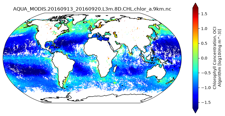
In this example, the image to be used is MODIS AQUA L3 8-day averaged 4km chlorophyll image for Sep 13-20, 2016 and the January 2020 monthly average for Rrs_412. First we need to search for that data. These data are hosted by the OB.DAAC. The earthaccess.search_datasets function queries the CMR for collections. To do this search we need to know something about the data information, particularly that we are looking for L3m or Level-3 mapped collections and MODIS AQUA.

results = earthaccess.search_datasets(
    keyword="L3m ocean color modis aqua chlorophyll",
    instrument="MODIS",
)

set((i.summary()["short-name"] for i in results))

{'MODISA_L3m_CHL', 'MODISA_L3m_CHL_NRT', 'MODIST_L3m_CHL'}

You will want to go on to https://search.earthdata.nasa.gov/ and enter the short names to read about each data collection. We want to use the MODISA_L3m_CHL data collection for our first plot. We can get the files (granules) in that collection with earthaccess.search_data().

tspan = ("2016-09-20", "2016-09-20")
results = earthaccess.search_data(
    short_name="MODISA_L3m_CHL",
    temporal=tspan,
)

Clearly, that’s too many granules for a single day! The OB.DAAC publishes multiple variants of a dataset under the same short name, and the only way to distinguish them is by the product or granule name. The CMR search allows a granule_name parameter with wildcards for this kind of filter. The strings we need to see in the granule name are “.8D” and “.9km” (the “.” is a separator used in granule names).

results = earthaccess.search_data(
    short_name="MODISA_L3m_CHL",
    granule_name="*.8D*.9km*",
    temporal=tspan,
)

results[0]

Data: AQUA_MODIS.20160913_20160920.L3m.8D.CHL.chlor_a.9km.nc

Size: 13.74 MB

Cloud Hosted: True

We need to check if the data are cloud-hosted. If they are and we are, we can load into memory directly without downloading. If they are not cloud-hosted, we need to download the data file.

if results[0].cloud_hosted:
    paths = earthaccess.open(results)
else:
    paths = earthaccess.download(results, "granules")

If you see HTTPFileSystem in the output when displaying paths, then earthaccess has determined that you do not have direct access to the NASA Earthdata Cloud. It may be wrong.

3. Plot Data#

array = np.log10(dataset["chlor_a"])
array.attrs.update(
    {
        "units": f'log10({dataset["chlor_a"].attrs["units"]})',
    }
)
crs_proj = cartopy.crs.Robinson()
crs_data = cartopy.crs.PlateCarree()

fig, ax = plt.subplots(figsize=(10, 5), subplot_kw={"projection": crs_proj})
plot = array.plot(x="lon", y="lat", cmap="jet", ax=ax, robust=True, transform=crs_data)
ax.coastlines()
ax.set_title(dataset.attrs["product_name"])
plt.show()

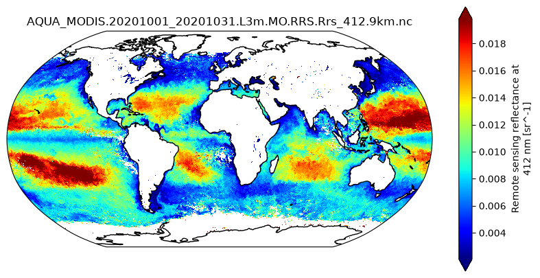
../../_images/90cdd5e9f2d7889acc30339aba5c89d5eda11cc7cd34da8cedb725e1fd07886e.png

Repeat these steps to map the monthly Rrs_412 dataset, a temporal average of cloud-free pixels, aggregated to 9km spatial resolution, for October 2020.

tspan = ("2020-10-01", "2020-10-01")
results = earthaccess.search_data(
    short_name="MODISA_L3m_RRS",
    granule_name="*.MO*.Rrs_412*.9km*",
    temporal=tspan,
)
if results[0].cloud_hosted:
    paths = earthaccess.open(results)
else:
    paths = earthaccess.download(results, "granules")

dataset = xr.open_dataset(paths[0])

fig, ax = plt.subplots(figsize=(10, 5), subplot_kw={"projection": crs_proj})
plot = dataset["Rrs_412"].plot(
    x="lon", y="lat", cmap="jet", robust=True, ax=ax, transform=crs_data
)
ax.coastlines()
ax.set_title(dataset.attrs["product_name"])
plt.show()

../../_images/33fbbb1a84e942b9bc89ecebf4c76c8e993b356e882502ff6e52c594d3c3bf39.png

You have completed the notebook on Level-3 mapped ocean color data from Aqua/MODIS.