

Visualize HARP2 CLOUD GPC Product#
Author(s): Chamara Rajapakshe (NASA, SSAI), Kirk Knobelspiesse (NASA), Andy Sayer (NASA, UMBC), Meng Gao (NASA, SSAI), Sean Foley (NASA, MSU)
Last updated: July 22, 2026
Summary#
This notebook summarizes how to access HARP2 GISS Polarimetric Cloud (GPC) products (CLOUD_GPC). Note that this notebook is based on an early preliminary version of the product and is therefore subject to future optimizations and changes.
Learning Objectives#
By the end of this notebook, you will understand:
How to acquire HARP2 Level-2 data
Available variables in the product
How to visualize variables
1. Setup#
Begin by importing all of the packages used in this notebook. If you followed the guidance on the Getting Started page, then the imports will be successful.
import cartopy.crs as ccrs
import earthaccess
import matplotlib.colors as mcolors
import matplotlib.pyplot as plt
import numpy as np
import pandas as pd
import xarray as xr
Global settings and variables used throughout the notebook.
plt.style.use("seaborn-v0_8-notebook")
pd.set_option("display.max_colwidth", 0)
projection = ccrs.PlateCarree()
Set (and optionally persist to your home directory as a “netrc” file) your Earthdata Login credentials.
auth = earthaccess.login()
2. Get Level-2 Data#
You can use PACE_HARP2_L2_CLOUD_GPC as the short name to get the most recent version available for the CLOUD_GPC provisional product at Level-2 for the HARP2 instrument. Add the Near Real Time (NRT) suffix for the most recent observations (i.e. PACE_HARP2_L2_CLOUD_GPC_NRT).
results = earthaccess.search_datasets(instrument="harp2")
for item in results:
    summary = item.summary()
    if "CLOUD" in summary["short-name"]:
        print(summary["short-name"])
PACE_HARP2_L2_CLOUD_GPC_NRT
PACE_HARP2_L2_CLOUD_GPC_NRT
PACE_HARP2_L2_CLOUD_GPC
PACE_HARP2_L2_CLOUD_GPC
PACE_HARP2_L3M_CLOUD_GPC_NRT
PACE_HARP2_L3M_CLOUD_GPC_NRT
PACE_HARP2_L3M_CLOUD_GPC
PACE_HARP2_L3M_CLOUD_GPC
Search for available granules within a time range and geospatial area of interest. The order of values in a “bounding_box” is always West (longitude), South (latitude), East (longitude), North (latitude). If you know the actual granule name, you can use “granule_name” explicitly. You may get multiple versions if you include a * instead of an explicit version.
results = earthaccess.search_data(
    short_name="PACE_HARP2_L2_CLOUD_GPC",
    granule_name='PACE_HARP2.20240904T205635.L2.CLOUD_GPC.V3*.nc',
)
for item in results:
    display(item)

paths = earthaccess.open(results)
Here we merge all the data groups together for convenience in data manipulations.
datatree = xr.open_datatree(paths[0])
dataset = xr.merge(datatree.to_dict().values())
dataset = dataset.set_coords(("latitude", "longitude"))
3. Understanding HARP2 L2.CLOUD_GPC Product Structure#
HARP2 CLOUD_GPC products provide descriptive metadata for the variables. However, given the early stage of the product, improvements and changes are expected in future versions.
def print_variable_description(datatree, variables, exclude=False):
    """
    Print a table of variables, units, and descriptions from the
    `geophysical_data` group of a DataTree-like object.

    Parameters
    ----------
    datatree : DataTree or dict-like
        Object containing a `geophysical_data` group with variables
        whose metadata are stored in `attrs` (e.g., `units` and `long_name`).
    variables: list of str
        Substrings used to filter variable names.
    exclude : bool, default False
        If False (default), only variables whose names contain any of the
        substrings in `ret_type_list` are shown. If True, show all others.

    Notes
    -----
    Long descriptions are wrapped to 100 characters; only the first line
    prints the variable name and units.
    """
    df = pd.DataFrame(columns=("Units", "Description"))
    for key, value in datatree["geophysical_data"].data_vars.items():
        # select based on inclusion (or exclusion) logic
        match = any(i in key for i in variables)
        if (match and not exclude) or (not match and exclude):
            units = value.attrs.get("units", "")
            desc = value.attrs.get("long_name", "")
            df.loc[key, :] = [units, desc]
    return df
Cloud Bow Retrievals#
One of the main retrieval techniques implemented is the parametric cloud bow retrieval method (Bréon & Goloub, 1998; Alexandrov et al., 2012). The phrase “cloud_bow” is appended to variable names, their corresponding diagnostic variables, and additional variables derived by combining them with OCI Level 2 products. For example, “cloud_bow_droplet_number_concentration_adiabatic” and “cloud_bow_liquid_water_path” are derived using the retrieved droplet size distributions along with OCI L2.CLOUD properties. Additional descriptions can be found in the file attributes as follows:
print_variable_description(datatree, ["bow"])
| Units | Description | |
|---|---|---|
| cloud_bow_droplet_effective_radius | um | Cloud droplet effective radius obtained using Cloud Bow. The bands used in the retrieval are (665). |
| cloud_bow_droplet_effective_radius_stddev | um | Standard deviation of cloud droplet effective radius obtained using Cloud Bow. |
| cloud_bow_droplet_effective_variance | 1 | Cloud droplet effective variance obtained using Cloud Bow. The bands used in the retrieval are (665). |
| cloud_bow_droplet_effective_variance_stddev | 1 | Standard deviation of cloud droplet effective variance obtained using Cloud Bow. |
| cloud_bow_rms | 1 | Root mean square of data fit to retrieved cloud droplet radius and variance obtained using Cloud Bow. |
| cloud_bow_fit_correlation | 1 | Correlation of data fit to retrieved cloud droplet radius and variance obtained using Cloud Bow. |
| cloud_bow_cirrus_correlation | 1 | Correlation of cirrus fit to retrieved cloud droplet radius and variance obtained using Cloud Bow. |
| cloud_bow_auxiliary_fit | 1 | Auxiliarly_fit parameters C, B, A, accounting for linear addition offset, Rayleigh term and P12 scaling, respectively (Alexandrov et al., RSE 2012, Eq. 3). One set per wavelength used in fit. |
| cloud_bow_extinction_cross_section_355nm | um2 | 355 nm extinction cross section based on 865 nm cloud bow effective radius and variance retrieval. |
| cloud_bow_extinction_cross_section_532nm | um2 | 532 nm extinction cross section based on 865 nm cloud bow effective radius and variance retrieval. |
| cloud_bow_lidar_ratio_355nm | sr | Ratio at 355 nm of extinction to backscatter at 180° scattering angle based on 865 nm cloud bow effective radius and variance retrieval. |
| cloud_bow_lidar_ratio_532nm | sr | Ratio at 532 nm of extinction to backscatter at 180° scattering angle based on 865 nm cloud bow effective radius and variance retrieval. |
| cloud_bow_droplet_number_concentration_adiabatic | # cm-3 | Cloud droplet number concentration assumes that the liquid water content is increasing with some assumed fraction of the adiabatic value. The assumptions and formulae used are summarized in Grosvenor et al. 2018 doi:10.1029/2017RG000593. |
| cloud_bow_liquid_water_path | g m-2 | Cloud liquid water path (LWP) is obtained from the product of optical thickness and droplet effective radius. It is assumed that the liquid water content is increasing linearly with height from cloud base. |
| cloud_bow_quality_retrieval_fail | 1 | If no bits are set (=0), the results are concluded OK. If bits are set, there is an issue with the retrieval. Fill value is used when there is no cloud or no data to check for cloud. |
RFT Retrievals#
The second retrieval technique is the Rainbow Fourier Transform (RFT) method (Alexandrov et al., 2012). The prefix cloud_rft is appended to variable names, their associated diagnostic variables, and other outputs generated by this algorithm.
print_variable_description(datatree, ["rft"])
| Units | Description | |
|---|---|---|
| cloud_rft_droplet_effective_radius_mode_0 | um | Cloud droplet modes effective radius from RFT retrievals for mode 0. |
| cloud_rft_droplet_effective_radius_mode_1 | um | Cloud droplet modes effective radius from RFT retrievals for mode 1. |
| cloud_rft_droplet_effective_variance_mode_0 | 1 | Cloud droplet modes effective variance from RFT retrievals for mode 0. |
| cloud_rft_droplet_effective_variance_mode_1 | 1 | Cloud droplet modes effective variance from RFT retrievals for mode 1. |
| cloud_rft_mode_fraction_0 | 1 | Cloud droplet modes fraction from RFT retrievals for mode 0. |
| cloud_rft_mode_fraction_1 | 1 | Cloud droplet modes fraction from RFT retrievals for mode 1. |
| cloud_rft_decomp_size_correlation | 1 | Correlation between the mode decomposition of the RFT and the size distribution. |
| cloud_rft_quality_retrieval_fail | 1 | If no bits are set (=0), the results are concluded OK. If bits are set, there is an issue with the retrieval. Fill value is used when there is no cloud or no data to check for cloud. |
Cloud Liquid Index Retrievals#
Cloud Bow Liquid Index (CLI) retrievals provide a measure of the fraction of a cloud top composed of liquid vs ice.
print_variable_description(datatree, ["index"], exclude=False)
| Units | Description | |
|---|---|---|
| cloud_liquid_index | 1 | Index indicating the strength of the primary rainbow in the observed polarized reflectances owing to scattering on liquid drops. A liquid index <0.3 is considered to exclude presence of liquid drops in the tops of the observed clouds, and thus indicates glaciated cloud tops (van Diedenhoven et al., JAS 2012). |
Additional Variables From OCI L2.CLOUD Products#
In addition to the main quantities retrieved by the algorithms, CLOUD_GPC also includes several commonly useful ancillary variables.
print_variable_description(datatree, ["index", "rft", "bow"], exclude=True)
| Units | Description | |
|---|---|---|
| cloud_top_altitude | m | Cloud top altitude |
| cloud_top_temperature | K | Air temperature at the cloud top |
| cloud_top_pressure | Pa | Air pressure at the cloud top |
| cloud_optical_thickness | 1 | Cloud optical thickness obtained from AUX file. |
| cloud_quality | 1 | If no bits are set (=0), the results are concluded OK. If bits are set, there is an issue with the retrieval. Fill value is used when there is no cloud or no data to check for cloud. |
4. Visulizing Variables#
def extremes_removed_limits(array):
    """
    Return a boolean mask indicating which elements of `array` are not extreme
    outliers based on the interquartile range (IQR) rule.

    Parameters
    ----------
    array : array-like
        Input numeric array.

    Returns
    -------
    tuple
        suggested min and max for axis limits in plots
    """
    q0, q1, q3, q4 = array.quantile([0, 0.25, 0.75, 1])
    vmin = q1 - 1.5 * (q3 - q1)
    vmax = q3 + 1.5 * (q3 - q1)
    return max(q0, vmin), min(q4, vmax)


def geo_axis_tags(ax, crs=ccrs.PlateCarree()):
    """
    Add coastlines and labeled latitude/longitude gridlines to a Cartopy axis.

    Parameters
    ----------
    ax : cartopy.mpl.geoaxes.GeoAxes
        Axes object on which to draw the gridlines and coastlines.
    crs : cartopy.crs.CRS, optional
        Coordinate reference system used for the gridlines.
        Default is a Plate Carrée projection with central longitude = 0.
    """
    gl = ax.gridlines(
        crs=crs,
        draw_labels=["left", "bottom"],
        xlabel_style={"size": 12, "color": "k"},
        ylabel_style={"size": 12, "color": "k"},
    )
    ax.coastlines()
    return
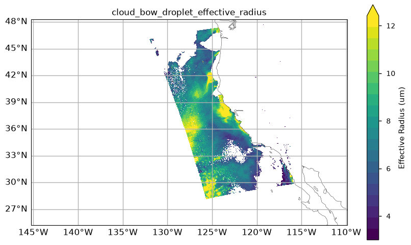
Here we visualize the effective radius retrieved using the cloud-bow (parametric) technique. The colorbar limits are adjusted based on the range of observed effective radii, excluding extreme values. Retrievals are only possible in the central portion of the HARP2 granule, where the required angular sampling for the cloud-bow and supernumerary-bow scattering angles is available. Retrieval failure flags, provided in the variable cloud_bow_quality_retrieval_fail, indicate the reasons for unsuccessful retrievals.
fig, ax = plt.subplots(figsize=(10, 6), subplot_kw={"projection": projection})
var = "cloud_bow_droplet_effective_radius"
array = dataset[var]
vmin, vmax = extremes_removed_limits(array)
cmap = plt.get_cmap("viridis", 20)
img = array.plot.pcolormesh(
    x="longitude",
    y="latitude",
    cmap=cmap,
    vmin=vmin,
    vmax=vmax,
)
img.colorbar.set_label("Effective Radius (um)")
ax.set_title(var, size=12)
geo_axis_tags(ax, projection)
plt.show()
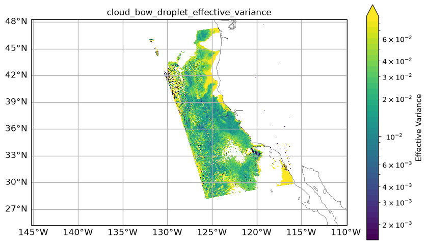
Cloud Effective Variance is a key parameter uniquely provided by polarimetry, and together with Cloud Effective Radius, it fully characterizes the modified gamma distribution of cloud droplet sizes. A logarithmic color scale is used to display its detailed variability.
fig, ax = plt.subplots(figsize=(10, 6), subplot_kw={"projection": projection})
var = "cloud_bow_droplet_effective_variance"
array = dataset[var]
vmin, vmax = extremes_removed_limits(array)
cmap = plt.get_cmap("viridis", 40)
norm = mcolors.LogNorm(vmin=vmin, vmax=vmax)
img = array.plot.pcolormesh(
    x="longitude",
    y="latitude",
    cmap=cmap,
    norm=norm,
)
img.colorbar.set_label("Effective Variance")
ax.set_title(var, size=12)
geo_axis_tags(ax)
plt.show()
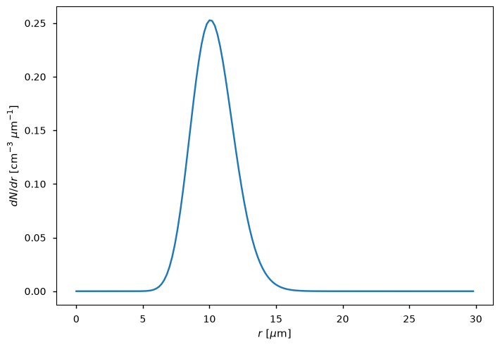
Cloud effective radius and variance in combination provide the full droplet size distribution in the form of a modified gamma distribution
def mod_gamma_norm(re, ve, r=np.arange(0, 30, 0.2)):
    '''
    Normalized modified gamma distribution for effective radius and variance.

    Parameters
    ----------
    re : float
        Effective radius in microns
    ve : float
        Effective variance
    r : ndarray, optional
        Radius array in microns (default: 0 to 30 μm in 0.2 μm steps)

    Returns
    -------
    ndarray
        Normalized distribution (Hansen and Travis, 1974)
    '''
    f = r**((1.0 - 3.0*ve)/ve) * np.exp(-r/(re*ve))
    C = np.trapezoid(f, r)
    return f / C
Apply the new mod_gamma_norm function to compute normalized modified gamma distribution.
radius = np.arange(0, 30, 0.2)  # droplet radius in μm
n_d = mod_gamma_norm(
    dataset['cloud_bow_droplet_effective_radius'][180, 250].values,
    dataset['cloud_bow_droplet_effective_variance'][180, 250].values,
    r=radius
)
The plot of the distribution of the radius looks like a gamma distribution, as expected.
plt.plot(radius, n_d)
plt.xlabel(r'$r$ [$\mu$m]')
plt.ylabel(r'$dN/dr$ [$\mathrm{cm}^{-3}$ $\mu\mathrm{m}^{-1}$]')
plt.show()
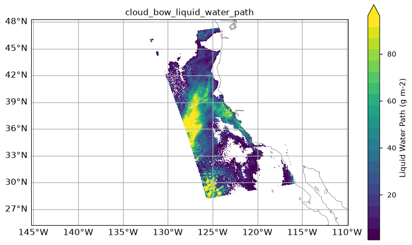
When the cloud effective radius is known, the cloud liquid water path can be derived by combining it with OCI’s cloud optical thickness retrievals. The GPC products include such derived cloud liquid water path fields based on the cloud-bow effective radius.
fig, ax = plt.subplots(figsize=(10, 6), subplot_kw={"projection": projection})
var = "cloud_bow_liquid_water_path"
array = dataset[var]
vmin, vmax = extremes_removed_limits(array)
cmap = plt.get_cmap("viridis", 20)
img = array.plot.pcolormesh(
    x="longitude",
    y="latitude",
    cmap=cmap,
    vmin=vmin,
    vmax=vmax,
)
img.colorbar.set_label("Liquid Water Path (g m-2)")
ax.set_title(var, size=12)
geo_axis_tags(ax)
plt.show()
5. Reference#
Breon, F.-M., & Doutriaux-Boucher, M. (2005). A comparison of cloud droplet radii measured from space. IEEE Transactions on Geoscience and Remote Sensing, 43(8), 1796–1805. https://doi.org/10.1109/TGRS.2005.852838
Alexandrov, M. D., Cairns, B., Emde, C., Ackerman, A. S., & Van Diedenhoven, B. (2012). Accuracy assessments of cloud droplet size retrievals from polarized reflectance measurements by the research scanning polarimeter. Remote Sensing of Environment, 125, 92–111. https://doi.org/10.1016/j.rse.2012.07.012
Van Diedenhoven, B., Fridlind, A. M., Ackerman, A. S., & Cairns, B. (2012). Evaluation of Hydrometeor Phase and Ice Properties in Cloud-Resolving Model Simulations of Tropical Deep Convection Using Radiance and Polarization Measurements. Journal of the Atmospheric Sciences, 69(11), 3290–3314. https://doi.org/10.1175/JAS-D-11-0314.1
Alexandrov, M. D., Cairns, B., & Mishchenko, M. I. (2012). Rainbow Fourier transform. Journal of Quantitative Spectroscopy and Radiative Transfer, 113(18), 2521–2535. https://doi.org/10.1016/j.jqsrt.2012.03.025
You have completed the notebook on HARP2 cloud products. May we suggest studying the notebook on HARP2 aerosol products?