Accessing the CLOSE dataset

Accessing the CLOSE dataset#

Author: Anna Windle (NASA GSFC, SSAI)

Last updated: July 10, 2026

Summary#

Accurate evaluation of satellite ocean color algorithms is fundamentally limited by the absence of comprehensive datasets in which the true ocean state is fully known. Here we present CLOSE: a Closed-Loop Ocean Simulation for Evaluation. The CLOSE dataset is provided in a realistic satellite instrument coordinate framework to support the development and assessment of retrieval algorithms for NASA’s Plankton, Aerosol, Cloud, ocean Ecosystem (PACE) mission.

The input data includes remote sensing reflectance (Rrs(λ)), inherent optical properties (IOPs), phytoplankton community composition (PCC), and associated environmental variables derived from the NASA Ocean Biogeochemical Model (NOBM) coupled to the Ocean-Atmosphere Spectral Irradiance Model (OASIM).

These data are used as input to the Python Top-Of-Atmosphere Simulation Tool (PyTOAST) to simulate Level-1B top-of-atmosphere radiances, which are subsequently processed to Level-2 ocean color products. This framework provides end-to-end traceability from modeled ocean variables to retrieved geophysical retrievals, providing a unique resource for robust algorithm development, validation, and uncertainty quantification.

This openly available dataset represents the first fully closed, spatially explicit simulation of PACE-like measurements, establishing a foundation for evaluation of atmospheric correction and bio-optical (empirical and semi-analytical) methods. It is designed to accelerate algorithm development, enhance confidence in satellite-derived products, and ultimately advance global ocean biogeochemical observing capabilities. More information on the CLOSE dataset can be found in this manuscript. (link to be added)

The entire CLOSE dataset is hosted and provided free of charge through the NASA Ocean Biology Distribution Active Archive Center (OB.DAAC). Data are available as NetCDF (.nc) files. The primary links for referencing these data are:

Data can be accessed via the OB.DAAC File Search. Click “Advanced” at the top, filter “Instrument” to “PACE-OCI” and filter through “Data Type”. The following are the Data Types for the CLOSE dataset:

PACE-OCI SIM PyTOAST Model Inputs for CLOSE
PACE-OCI SIM PyTOAST Level-1B Observations for CLOSE
PACE-OCI SIM PyTOAST Level-2 Observations for CLOSE
PACE-OCI SIM PyTOAST Level-3 Binned Observations for CLOSE
PACE-OCI SIM PyTOAST Level-3 Mapped Observations for CLOSE

You can leave all other selections the default, and press “Submit”. This will take you to a page where you can download the files directly. You can also use the command line retireval methods, examples are shown on the File Search website.

This tutorial demonstrates how to access CLOSE data using command line methods within a Jupyter notebook.

Learning Objectives#

At the end of this notebook, you will know how to:

Find and download CLOSE data from OB.DAAC
Use Python requests to query the OB.DAAC File Search using the API

1. Setup#

Begin by importing all of the packages used in this notebook.

from pathlib import Path

import matplotlib.pyplot as plt
import numpy as np
import requests
import xarray as xr
from tqdm.notebook import tqdm

2. Query OB.DAAC File Search#

We can query the OB.DAAC File Search using the API, which has documentation for all available parameters. Let’s start by counting how many files exist for several CLOSE product types on our target date of 2025-03-15. You can change this date to any of the other dates for which CLOSE data are available:

2025-01-15
2025-03-15
2025-06-15
2024-09-15

The URL for the API is the same as the OB.DAAC File Search form:

url = "https://oceandata.sci.gsfc.nasa.gov/file_search"

These parameters are going to be sent with each of our queries:

sensor="PACE-OCI" → the name of the sensor
sdate → search start date
edate → search end date
results_as_file=1 → return a plain text list of matching filenames

common_params = {
    "sensor": "PACE-OCI",
    "sdate": "2025-03-15T00:00:00",
    "edate": "2025-03-15T23:59:59",
    "results_as_file": 1,
}

Each dataset we need has an OB.DAAC-specific identifier, which can be found in the documentation for dtid.

datasets = {
    "Model Input": 165,
    "L1B": 164,
    "L2": 161,
    "L3M": 163,
}

We can now make POST requests for each dataset, and build up a list of files to download. Depending on the current load on the File Search database, this step may take anywhere from a few seconds to several minutes.

files = {}
for name, dtid in datasets.items():
    response = requests.post(url, data={**common_params, "dtid": dtid})
    response.raise_for_status()
    lines = list(response.iter_lines(decode_unicode=True))
    files[name] = lines
    print(f"Total number of {name} files: {len(lines)}")

Total number of Model Input files: 148
Total number of L1B files: 148
Total number of L2 files: 148
Total number of L3M files: 1

3. Download data#

In this example, we grab one file for each data product type. We are downloading files corresponding to a date and granule discussed in the manuscript: Granule B in Figure 1. We can download each file from lists in the files dictionary, and save it to a local directory called CLOSE_data. You can change this directory name to any location or folder name that best fits your workflow.

url = "https://oceandata.sci.gsfc.nasa.gov/getfile/"
data = Path("CLOSE_data")
data.mkdir(parents=True, exist_ok=True)
session = requests.Session()

target_time = "20250315T152616"
target_date = "20250315"

paths = {}
for name in tqdm(files):
    example_files = [f for f in files[name] if target_time in str(f) or (name== "L3M" and target_date in str(f))]
    example_file = Path(example_files[0])
    with session.get(f"{url}/{example_file}", stream=True) as r:
        r.raise_for_status()
        with (data / example_file).open("wb") as f:
            f.writelines(r.iter_content(chunk_size=2**20))
    paths[name] = data / example_file

4. Open and plot the data#

Now that the data have been downloaded locally, we can open it as an xarray dataset and prepare it for subsequent analysis.

model_inputs = xr.open_dataset(paths["Model Input"])
model_inputs = model_inputs.set_coords(("longitude", "latitude"))

l1b = xr.open_datatree(paths["L1B"])
l1b = xr.merge(l1b.to_dict().values())
l1b = l1b.set_coords(("longitude", "latitude"))

l2 = xr.open_datatree(paths["L2"], decode_timedelta=False)
l2 = xr.merge(l2.to_dict().values())
l2 = l2.set_coords(("longitude", "latitude"))

l3m = xr.open_dataset(paths["L3M"])

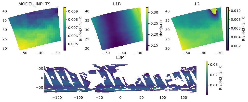
Let’s plot either remote sensing reflectance (Rrs) or top-of-atmopshere reflectance (rhot) from each file:

fig = plt.figure(figsize=(10, 4), constrained_layout=True)
gs = fig.add_gridspec(2, 3)

ax1 = fig.add_subplot(gs[0, 0])
ax2 = fig.add_subplot(gs[0, 1])
ax3 = fig.add_subplot(gs[0, 2])
ax4 = fig.add_subplot(gs[1, 0:3])

m1 = (
    model_inputs["Rrs"]
    .sel({"wavelength": 442}, method="nearest")
    .plot(ax=ax1, x="longitude", y="latitude", add_colorbar=True)
)
ax1.set_title("MODEL_INPUTS")

m2 = (
    l1b["rhot_blue"]
    .sel({"blue_bands": 53})
    .plot(ax=ax2, x="longitude", y="latitude", add_colorbar=True)
)
ax2.set_title("L1B")

m3 = (
    l2["Rrs"]
    .sel({"wavelength_3d": 442}, method="nearest")
    .plot(ax=ax3, x="longitude", y="latitude", add_colorbar=True)
)
ax3.set_title("L2")

m4 = (
    l3m["Rrs"]
    .sel({"wavelength": 442}, method="nearest")
    .plot(ax=ax4, x="lon", y="lat", add_colorbar=True)
)
ax4.set_title("L3M")

# --- Two-line colorbar labels ---
m1.colorbar.set_label("Rrs(442) (sr⁻¹)")
m2.colorbar.set_label("Rhot(442)")
m3.colorbar.set_label("Rrs(442) (sr⁻¹)")
m4.colorbar.set_label("Rrs(442) (sr⁻¹)")

for ax in [ax1, ax2, ax3, ax4]:
    ax.set_xlabel("")
    ax.set_ylabel("")
    ax.tick_params(length=0)
    for spine in ax.spines.values():
        spine.set_visible(False)

# shift bottom row to the right and down
pos = ax4.get_position()
ax4.set_position([pos.x0 + 0.05, pos.y0 - 0.07, pos.width, pos.height])

# shift colorbar
cbar = m4.colorbar
cbar.ax.set_position(
    [
        cbar.ax.get_position().x0 + 0.05,
        cbar.ax.get_position().y0 - 0.07,
        cbar.ax.get_position().width,
        cbar.ax.get_position().height,
    ]
)

plt.show()

../../_images/9ac17be3464f03f5d42c050ce67d91aef84b28a231e997d9948fba4db5fea164.png

This code can be easily adapted to download multiple granules. By downloading the complete set of associated files, you can examine each stage of the processing chain and explore how the data evolve from one product level to the next.

5. Example of comparing input and output geophysical data products#

By providing known “truth” fields in native satellite geometry, CLOSE offers a powerful testbed for atmospheric correction, bio-optical inversion, and emerging machine learning approaches.

Here is an example of comparing input Chl a (derived mechanistically from NOBM) to output Chl a derived from NASA OB.DAAC (see Chl a ATBD).

plot = model_inputs["chlor_a"].plot.hist(
    bins=50,
    range=[0.007, 0.4],
    alpha=0.4,
    label="MODEL_INPUTS Chl a",
    color="blue",
)

plot = l2["chlor_a"].plot.hist(
    bins=50,
    range=[0.007, 0.4],
    alpha=0.4,
    label="L2 Chl a",
    color="red",
)

median_model_inputs_chl = np.nanmedian(model_inputs["chlor_a"].values)
median_l2_chl = np.nanmedian(l2["chlor_a"].values)
print(median_model_inputs_chl, median_l2_chl)

plt.axvline(
    median_model_inputs_chl,
    color="blue",
    linewidth=2,
    label=f"MODEL_INPUTS Chl median= {median_model_inputs_chl:.2f}",
)
plt.axvline(
    median_l2_chl,
    color="red",
    linestyle="--",
    linewidth=2,
    label=f"L2 Chl median= {median_l2_chl:.2f}",
)

plt.xlabel("Chl a (mg m$^{-3}$)", fontsize=10)
plt.ylabel("Frequency", fontsize=10)

plt.legend(frameon=False)
plt.show()

0.089011624 0.09519954

../../_images/6cdaf973bfafe0e8fb5621bf99f830b1a33c98e4623192cdd0ee7f05739c7b96.png

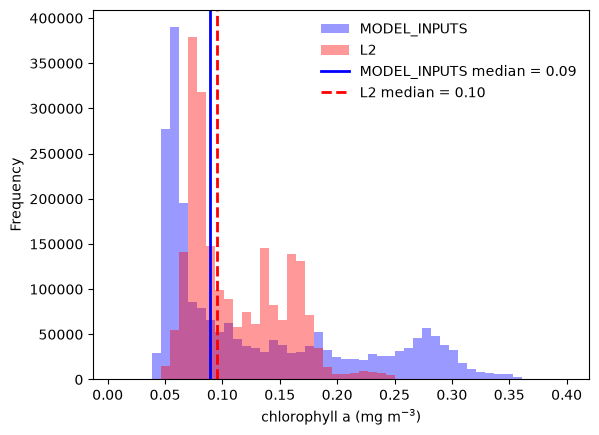
Overall, Chl a distributions are similar, with only slight differences in their medians. This example evaluates the standard Chl a algorithm, but it could be replaced with any alternative algorithm to assess how well its output compares to the input (“truth”) Chl a. The same approach can be applied to other data products as well.

You have completed the notebook on “Accessing the CLOSE Dataset”!