

Applying Spectral Derivative Pigments (SDP) Phytoplankton Community Composition Algorithm to OCI data#
Author(s): Anna Windle (NASA, SSAI), Ian Carroll (NASA, UMBC)
Adapted from code developed by: Max Danenhower (Bowdoin College), Sasha Kramer (Boston University)
Last updated: July 24, 2026
The following notebooks are prerequisites for this tutorial.
Learn with OCI: Data Access
An Earthdata Login account is required to access data from the NASA Earthdata system, including NASA ocean color data.
Summary#
This notebook applies the coefficients generated from a principal components regression model trained on in situ data described in Kramer et al., 2022 to estimate phytoplankton pigment concentrations from the second derivative of a spectral Rrs residual generated from PACE OCI Rrs data. This algorithm, called Spectral Derivative Pigments (SDP), is currently being implemented in OBPG’s OCSSW software. This work was originally developed in MATLAB by Sasha Kramer and subsequently translated to Python by Max Danenhower. This tutorial demonstrates how to apply the Python SDP algorithm to Level-2 (L2) PACE OCI data.
Learning Objectives#
At the end of this notebook you will know:
About searching for auxiliary data for the SDP algorithm
How to run the SDP algorithm on PACE OCI L2 data
1. Setup#
The SDP algorithm has been implemented as a Python package, so it can be easily installed, imported, and reused.
While the package is not on PyPI or conda-forge, it can be installed directly from the source repository on GitHub.
If you have followed the setup instructions, then sdp is available to import along with the other packages needed for this notebook.
import cartopy.crs as ccrs
import cartopy.feature as cfeature
import earthaccess
import matplotlib.pyplot as plt
import numpy as np
import xarray as xr
from sdp import sdp_from_pace
Set (and persist to your home directory on the host, if needed) your Earthdata Login credentials.
auth = earthaccess.login()
Assign “global” variables, which could be anything you want to define once and use consistently.
crs = ccrs.PlateCarree()
2. Access and open data#
We need the following data to run SDP:
Remote sensing reflectance (Rrs): PACE OCI L2 AOP data products
Sea surface salinity (SSS): JPL SMAP-SSS V5.0 CAP, 8-day running mean, level 3 mapped product from the NASA Soil Moisture Active Passive (SMAP) observatory
Sea surface temperature (SST): Group for High Resolution Sea Surface Temperature (GHRSST) Level 4 sea surface temperature
We can use earthaccess to find PACE OCI L2 data, checking in both the near-real-time and refined collections.
tspan = ("2026-05-05 17:35", "2026-05-05 17:35")
results = earthaccess.search_data(
    short_name=["PACE_OCI_L2_AOP_NRT", "PACE_OCI_L2_AOP"],
    temporal=tspan,
    count=1,
)
paths = earthaccess.open(results)
Let’s take a quick look at Rrs at 500nm:
datatree = xr.open_datatree(paths[-1])
rrs = datatree["geophysical_data"]["Rrs"]
for item in ("longitude", "latitude"):
    rrs[item] = datatree["navigation_data"][item]
rrs
<xarray.DataArray 'Rrs' (number_of_lines: 1710, pixels_per_line: 1272,
                         wavelength: 172)> Size: 1GB
[374120640 values with dtype=float32]
Coordinates:
    longitude   (number_of_lines, pixels_per_line) float32 9MB ...
    latitude    (number_of_lines, pixels_per_line) float32 9MB ...
  * wavelength  (wavelength) float32 688B 346.0 348.5 350.9 ... 716.8 719.3
Dimensions without coordinates: number_of_lines, pixels_per_line
Attributes:
    long_name:      Remote sensing reflectance
    units:          sr^-1
    standard_name:  surface_ratio_of_upwelling_radiance_emerging_from_sea_wat...
    valid_min:      -30000
valid_max: 25000fig, ax = plt.subplots(figsize=(8, 6), subplot_kw={"projection": crs})
da = rrs.sel({"wavelength": 500}, method="nearest")
da.plot(
x="longitude",
y="latitude",
vmin=0,
vmax=0.008,
ax=ax,
cbar_kwargs={"label": "Rrs ($sr^{-1}$)"},
)
ax.coastlines(resolution="10m")
ax.add_feature(cfeature.BORDERS, linestyle=":")
ax.gridlines(
draw_labels=["left", "bottom"],
linewidth=0.5,
color="gray",
alpha=0.5,
linestyle="--",
)
plt.show()
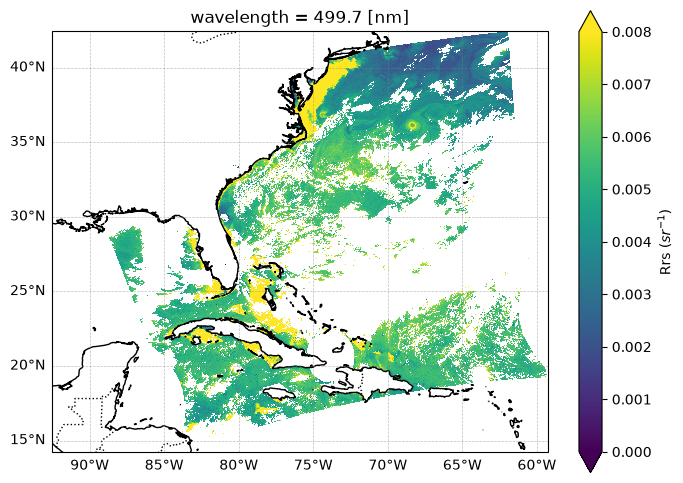
Now, we can use sdp_from_pace to calculate phytoplankton pigment concentrations for this data. Let’s take a look at the docstring for this function:
?sdp_from_pace
You can see that this function accepts a bbox parameter for limiting calculations to a bounding box. The default is bbox=None, meaning the algorithm is applied to every single pixel in the L2 granule, which can take a significnat amount of time and may exceed available system memory. We will supply the bbox parameter with the following coordinates: 38 N, 35 S, -70 E, -67 W.
bbox = (-73.5, 37.5, -67, 40.5)

lon_min, lat_min, lon_max, lat_max = bbox
rect_lon = [lon_min, lon_max, lon_max, lon_min, lon_min]
rect_lat = [lat_min, lat_min, lat_max, lat_max, lat_min]
ax.plot(rect_lon, rect_lat, color="red", linewidth=2)

fig
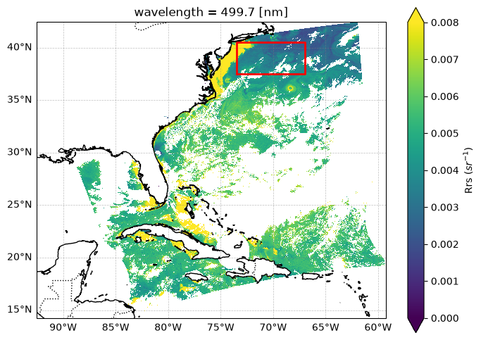
We need to find corresponding sea-surface salinity and temperature data for the SDP algorithm.
results = earthaccess.search_data(
    short_name="SMAP_JPL_L3_SSS_CAP_8DAY-RUNNINGMEAN_V5",
    temporal=tspan,
    count=1,
)
sss_paths = earthaccess.open(results)
results = earthaccess.search_data(
    short_name="MUR-JPL-L4-GLOB-v4.1",
    temporal=tspan,
    count=1,
)
sst_paths = earthaccess.open(results)
3. Run SDP on L2 Data#
Now we’re ready to run SDP. Let’s name what we want the outfile to be:
output_file = paths[-1].full_name.split("/")[-1]
output_file = output_file.replace(".nc", "_SDP_pigments.nc")
output_file
'PACE_OCI.20260505T173406.L2.OC_AOP.V3_2.NRT_SDP_pigments.nc'
And let’s run it! There will be some RuntimeWarnings that need to be considered.
sdp_from_pace(
    paths[-1],
    output_file,
    sss_file=sss_paths[-1],
    sst_file=sst_paths[-1],
    bbox=bbox,
)
starting interpolation
north 40.5 south 37.5 east -67 west -73.5
interpolation complete: 5.368409356015036
rrs_interp shape: (110331, 374)
(70338,) (70338,) (70338, 301)
0
calculating residuals
ray availble resources {'CPU': 3.0, 'object_store_memory': 1384721203.0, 'node:__internal_head__': 1.0, 'node:192.168.0.152': 1.0, 'memory': 3231016141.0}
(raylet) Task run_batch failed due to oom. There are infinite oom retries remaining, so the task will be retried. Error: 3 worker(s) were killed due to the node running low on memory. Memory on the node (IP: 192.168.0.152, ID: b2968ae152bd9e41c3ecbe45dfd2121edf417729384fcc77e922e7a2) was 13.87GB / 14.54GB (0.954073); OOM kill reason: Memory usage 14850879488B exceeded threshold of 14830787584B (95.0% of 15611355136B total); Object store memory usage: [- objects spillable: 117; - bytes spillable: 614141853; - objects unsealed: 0; - bytes unsealed: 0; - objects in use: 129; - bytes in use: 677658195; - objects evictable: 0; - bytes evictable: 0; ; - objects created by worker: 129; - bytes created by worker: 677658195; - objects restored: 0; - bytes restored: 0; - objects received: 0; - bytes received: 0; - objects errored: 0; - bytes errored: 0; ; Eviction Stats:; (global lru) capacity: 1384721203; (global lru) used: 0%; (global lru) num objects: 0; (global lru) num evictions: 0; (global lru) bytes evicted: 0]; Ray killed 3 worker(s) based on the killing policy; Considered workers: [; Selected to kill: (Task: job ID=01000000, lease ID=0300000001000000ffffffffffffffffffffffffffffffffffffffffffffffff, task name=run_batch, required resources={CPU: 1}, pid=9336, actual memory used=0.19GB, worker ID=66eb50285c82c51b25bba18e44552225df3de9c511993921fc4390dd); Selected to kill: (Task: job ID=01000000, lease ID=0200000001000000ffffffffffffffffffffffffffffffffffffffffffffffff, task name=run_batch, required resources={CPU: 1}, pid=9335, actual memory used=0.19GB, worker ID=f803b143e288bf95a2b6f81a77b2c7b678d154f5879f2f63b9b2df3c); Selected to kill: (Task: job ID=01000000, lease ID=0100000001000000ffffffffffffffffffffffffffffffffffffffffffffffff, task name=run_batch, required resources={CPU: 1}, pid=9337, actual memory used=0.19GB, worker ID=7403f8d7878d2c64cbc2b3a38e348fba165ae075a3648c8d738a5b99)]; Total non-selected idle workers: 0; Total non-selected idle workers USS bytes: 0.00GB; To see more information about memory usage on this node, use `ray logs raylet.out -ip 192.168.0.152`; Top 10 memory users: PID	MEM(GB)	COMMAND; 4447	3.97	l2gen par=l2gen_iop_mod.par; 8999	2.87	/srv/conda/envs/notebook/bin/python -m ipykernel_launcher -f /tmp/tmp6f8ce34d.json --HistoryManager....; 9071	2.73	/srv/conda/envs/notebook/bin/python -m ipykernel_launcher -f /tmp/tmpq2pf8aw1.json --HistoryManager....; 1551	0.84	/srv/conda/envs/notebook/bin/python -m ipykernel_launcher -f /tmp/tmp83fyr4x9.json --HistoryManager....; 10035	0.52	/srv/conda/envs/notebook/bin/python -m ipykernel_launcher -f /tmp/tmpkhmbxbav.json --HistoryManager....; 25	0.22	/srv/conda/envs/notebook/bin/python3.13 /srv/conda/envs/notebook/bin/jupyterhub-singleuser; 9336	0.19	ray::run_batch; 9335	0.19	ray::run_batch; 9337	0.19	ray::run_batch; 731	0.10	/srv/conda/envs/notebook/bin/python /srv/conda/envs/notebook/bin/jcache project -p docs/_cache execu...; Refer to the documentation on how to address the out of memory issue: https://docs.ray.io/en/latest/ray-core/scheduling/ray-oom-prevention.html. Consider provisioning more memory on this node or reducing task parallelism by requesting more CPUs per task. To adjust the kill threshold, set the environment variable `RAY_memory_usage_threshold` when starting Ray. To disable worker killing, set the environment variable `RAY_memory_monitor_refresh_ms` to zero. Since 2.56, Ray updated the oom killing policy to enabling killing multiple workers and selecting workers based on the time since the task start executing. To revert to the legacy policy of determining worker to oom kill based on owner group size or only selecting a single worker to kill at a time, set the environment variable `RAY_worker_killing_policy_by_group` to true before starting Ray. If the idle workers have a non-trivial memory footprint at the time of OOM (check OOM log for non-selected idle workers), consider setting the environment variable `RAY_idle_worker_killing_memory_threshold_bytes` to a lower value to consider idle workers with lower memory footprint for killing.
(raylet) Task run_batch failed due to oom. There are infinite oom retries remaining, so the task will be retried. Error: 3 worker(s) were killed due to the node running low on memory. Memory on the node (IP: 192.168.0.152, ID: b2968ae152bd9e41c3ecbe45dfd2121edf417729384fcc77e922e7a2) was 14.30GB / 14.54GB (0.983411); OOM kill reason: Memory usage 15132717056B exceeded threshold of 14830787584B (95.0% of 15611355136B total); Object store memory usage: [- objects spillable: 117; - bytes spillable: 614141853; - objects unsealed: 0; - bytes unsealed: 0; - objects in use: 129; - bytes in use: 677658195; - objects evictable: 0; - bytes evictable: 0; ; - objects created by worker: 129; - bytes created by worker: 677658195; - objects restored: 0; - bytes restored: 0; - objects received: 0; - bytes received: 0; - objects errored: 0; - bytes errored: 0; ; Eviction Stats:; (global lru) capacity: 1384721203; (global lru) used: 0%; (global lru) num objects: 0; (global lru) num evictions: 0; (global lru) bytes evicted: 0]; Ray killed 3 worker(s) based on the killing policy; Considered workers: [; Selected to kill: (Task: job ID=01000000, lease ID=0600000001000000ffffffffffffffffffffffffffffffffffffffffffffffff, task name=run_batch, required resources={CPU: 1}, pid=10618, actual memory used=0.12GB, worker ID=c790c5a4a3b08446fcd84c6bb8827a8046cb30c0f2d4176f0216b123); Selected to kill: (Task: job ID=01000000, lease ID=0500000001000000ffffffffffffffffffffffffffffffffffffffffffffffff, task name=run_batch, required resources={CPU: 1}, pid=10617, actual memory used=0.11GB, worker ID=1a6c55f384cc8a34223d304001390a1b5172409ab68d576d09eee70b); Selected to kill: (Task: job ID=01000000, lease ID=0400000001000000ffffffffffffffffffffffffffffffffffffffffffffffff, task name=run_batch, required resources={CPU: 1}, pid=10619, actual memory used=0.12GB, worker ID=d60f6154bcb04618d0ac0a13a8786235363634c8be0340aca22503dd)]; Total non-selected idle workers: 0; Total non-selected idle workers USS bytes: 0.00GB; To see more information about memory usage on this node, use `ray logs raylet.out -ip 192.168.0.152`; Top 10 memory users: PID	MEM(GB)	COMMAND; 4447	3.97	l2gen par=l2gen_iop_mod.par; 8999	2.94	/srv/conda/envs/notebook/bin/python -m ipykernel_launcher -f /tmp/tmp6f8ce34d.json --HistoryManager....; 10035	2.12	/srv/conda/envs/notebook/bin/python -m ipykernel_launcher -f /tmp/tmpkhmbxbav.json --HistoryManager....; 9071	1.76	/srv/conda/envs/notebook/bin/python -m ipykernel_launcher -f /tmp/tmpq2pf8aw1.json --HistoryManager....; 1551	0.84	/srv/conda/envs/notebook/bin/python -m ipykernel_launcher -f /tmp/tmp83fyr4x9.json --HistoryManager....; 25	0.22	/srv/conda/envs/notebook/bin/python3.13 /srv/conda/envs/notebook/bin/jupyterhub-singleuser; 10618	0.12	ray::IDLE; 10619	0.12	ray::IDLE; 10617	0.11	ray::IDLE; 731	0.10	/srv/conda/envs/notebook/bin/python /srv/conda/envs/notebook/bin/jcache project -p docs/_cache execu...; Refer to the documentation on how to address the out of memory issue: https://docs.ray.io/en/latest/ray-core/scheduling/ray-oom-prevention.html. Consider provisioning more memory on this node or reducing task parallelism by requesting more CPUs per task. To adjust the kill threshold, set the environment variable `RAY_memory_usage_threshold` when starting Ray. To disable worker killing, set the environment variable `RAY_memory_monitor_refresh_ms` to zero. Since 2.56, Ray updated the oom killing policy to enabling killing multiple workers and selecting workers based on the time since the task start executing. To revert to the legacy policy of determining worker to oom kill based on owner group size or only selecting a single worker to kill at a time, set the environment variable `RAY_worker_killing_policy_by_group` to true before starting Ray. If the idle workers have a non-trivial memory footprint at the time of OOM (check OOM log for non-selected idle workers), consider setting the environment variable `RAY_idle_worker_killing_memory_threshold_bytes` to a lower value to consider idle workers with lower memory footprint for killing.
(raylet) Task run_batch failed due to oom. There are infinite oom retries remaining, so the task will be retried. Error: 3 worker(s) were killed due to the node running low on memory. Memory on the node (IP: 192.168.0.152, ID: b2968ae152bd9e41c3ecbe45dfd2121edf417729384fcc77e922e7a2) was 13.87GB / 14.54GB (0.954073); OOM kill reason: Memory usage 14850879488B exceeded threshold of 14830787584B (95.0% of 15611355136B total); Object store memory usage: [- objects spillable: 117; - bytes spillable: 614141853; - objects unsealed: 0; - bytes unsealed: 0; - objects in use: 129; - bytes in use: 677658195; - objects evictable: 0; - bytes evictable: 0; ; - objects created by worker: 129; - bytes created by worker: 677658195; - objects restored: 0; - bytes restored: 0; - objects received: 0; - bytes received: 0; - objects errored: 0; - bytes errored: 0; ; Eviction Stats:; (global lru) capacity: 1384721203; (global lru) used: 0%; (global lru) num objects: 0; (global lru) num evictions: 0; (global lru) bytes evicted: 0]; Ray killed 3 worker(s) based on the killing policy; Considered workers: [; Selected to kill: (Task: job ID=01000000, lease ID=0300000001000000ffffffffffffffffffffffffffffffffffffffffffffffff, task name=run_batch, required resources={CPU: 1}, pid=9336, actual memory used=0.19GB, worker ID=66eb50285c82c51b25bba18e44552225df3de9c511993921fc4390dd); Selected to kill: (Task: job ID=01000000, lease ID=0200000001000000ffffffffffffffffffffffffffffffffffffffffffffffff, task name=run_batch, required resources={CPU: 1}, pid=9335, actual memory used=0.19GB, worker ID=f803b143e288bf95a2b6f81a77b2c7b678d154f5879f2f63b9b2df3c); Selected to kill: (Task: job ID=01000000, lease ID=0100000001000000ffffffffffffffffffffffffffffffffffffffffffffffff, task name=run_batch, required resources={CPU: 1}, pid=9337, actual memory used=0.19GB, worker ID=7403f8d7878d2c64cbc2b3a38e348fba165ae075a3648c8d738a5b99)]; Total non-selected idle workers: 0; Total non-selected idle workers USS bytes: 0.00GB; To see more information about memory usage on this node, use `ray logs raylet.out -ip 192.168.0.152`; Top 10 memory users: PID	MEM(GB)	COMMAND; 4447	3.97	l2gen par=l2gen_iop_mod.par; 8999	2.87	/srv/conda/envs/notebook/bin/python -m ipykernel_launcher -f /tmp/tmp6f8ce34d.json --HistoryManager....; 9071	2.73	/srv/conda/envs/notebook/bin/python -m ipykernel_launcher -f /tmp/tmpq2pf8aw1.json --HistoryManager....; 1551	0.84	/srv/conda/envs/notebook/bin/python -m ipykernel_launcher -f /tmp/tmp83fyr4x9.json --HistoryManager....; 10035	0.52	/srv/conda/envs/notebook/bin/python -m ipykernel_launcher -f /tmp/tmpkhmbxbav.json --HistoryManager....; 25	0.22	/srv/conda/envs/notebook/bin/python3.13 /srv/conda/envs/notebook/bin/jupyterhub-singleuser; 9336	0.19	ray::run_batch; 9335	0.19	ray::run_batch; 9337	0.19	ray::run_batch; 731	0.10	/srv/conda/envs/notebook/bin/python /srv/conda/envs/notebook/bin/jcache project -p docs/_cache execu...; Refer to the documentation on how to address the out of memory issue: https://docs.ray.io/en/latest/ray-core/scheduling/ray-oom-prevention.html. Consider provisioning more memory on this node or reducing task parallelism by requesting more CPUs per task. To adjust the kill threshold, set the environment variable `RAY_memory_usage_threshold` when starting Ray. To disable worker killing, set the environment variable `RAY_memory_monitor_refresh_ms` to zero. Since 2.56, Ray updated the oom killing policy to enabling killing multiple workers and selecting workers based on the time since the task start executing. To revert to the legacy policy of determining worker to oom kill based on owner group size or only selecting a single worker to kill at a time, set the environment variable `RAY_worker_killing_policy_by_group` to true before starting Ray. If the idle workers have a non-trivial memory footprint at the time of OOM (check OOM log for non-selected idle workers), consider setting the environment variable `RAY_idle_worker_killing_memory_threshold_bytes` to a lower value to consider idle workers with lower memory footprint for killing. [repeated 2x across cluster] (Ray deduplicates logs by default. Set RAY_DEDUP_LOGS=0 to disable log deduplication, or see https://docs.ray.io/en/master/ray-observability/user-guides/configure-logging.html#log-deduplication for more options.)
(raylet) Task run_batch failed due to oom. There are infinite oom retries remaining, so the task will be retried. Error: 3 worker(s) were killed due to the node running low on memory. Memory on the node (IP: 192.168.0.152, ID: b2968ae152bd9e41c3ecbe45dfd2121edf417729384fcc77e922e7a2) was 14.30GB / 14.54GB (0.983411); OOM kill reason: Memory usage 15132717056B exceeded threshold of 14830787584B (95.0% of 15611355136B total); Object store memory usage: [- objects spillable: 117; - bytes spillable: 614141853; - objects unsealed: 0; - bytes unsealed: 0; - objects in use: 129; - bytes in use: 677658195; - objects evictable: 0; - bytes evictable: 0; ; - objects created by worker: 129; - bytes created by worker: 677658195; - objects restored: 0; - bytes restored: 0; - objects received: 0; - bytes received: 0; - objects errored: 0; - bytes errored: 0; ; Eviction Stats:; (global lru) capacity: 1384721203; (global lru) used: 0%; (global lru) num objects: 0; (global lru) num evictions: 0; (global lru) bytes evicted: 0]; Ray killed 3 worker(s) based on the killing policy; Considered workers: [; Selected to kill: (Task: job ID=01000000, lease ID=0600000001000000ffffffffffffffffffffffffffffffffffffffffffffffff, task name=run_batch, required resources={CPU: 1}, pid=10618, actual memory used=0.12GB, worker ID=c790c5a4a3b08446fcd84c6bb8827a8046cb30c0f2d4176f0216b123); Selected to kill: (Task: job ID=01000000, lease ID=0500000001000000ffffffffffffffffffffffffffffffffffffffffffffffff, task name=run_batch, required resources={CPU: 1}, pid=10617, actual memory used=0.11GB, worker ID=1a6c55f384cc8a34223d304001390a1b5172409ab68d576d09eee70b); Selected to kill: (Task: job ID=01000000, lease ID=0400000001000000ffffffffffffffffffffffffffffffffffffffffffffffff, task name=run_batch, required resources={CPU: 1}, pid=10619, actual memory used=0.12GB, worker ID=d60f6154bcb04618d0ac0a13a8786235363634c8be0340aca22503dd)]; Total non-selected idle workers: 0; Total non-selected idle workers USS bytes: 0.00GB; To see more information about memory usage on this node, use `ray logs raylet.out -ip 192.168.0.152`; Top 10 memory users: PID	MEM(GB)	COMMAND; 4447	3.97	l2gen par=l2gen_iop_mod.par; 8999	2.94	/srv/conda/envs/notebook/bin/python -m ipykernel_launcher -f /tmp/tmp6f8ce34d.json --HistoryManager....; 10035	2.12	/srv/conda/envs/notebook/bin/python -m ipykernel_launcher -f /tmp/tmpkhmbxbav.json --HistoryManager....; 9071	1.76	/srv/conda/envs/notebook/bin/python -m ipykernel_launcher -f /tmp/tmpq2pf8aw1.json --HistoryManager....; 1551	0.84	/srv/conda/envs/notebook/bin/python -m ipykernel_launcher -f /tmp/tmp83fyr4x9.json --HistoryManager....; 25	0.22	/srv/conda/envs/notebook/bin/python3.13 /srv/conda/envs/notebook/bin/jupyterhub-singleuser; 10618	0.12	ray::IDLE; 10619	0.12	ray::IDLE; 10617	0.11	ray::IDLE; 731	0.10	/srv/conda/envs/notebook/bin/python /srv/conda/envs/notebook/bin/jcache project -p docs/_cache execu...; Refer to the documentation on how to address the out of memory issue: https://docs.ray.io/en/latest/ray-core/scheduling/ray-oom-prevention.html. Consider provisioning more memory on this node or reducing task parallelism by requesting more CPUs per task. To adjust the kill threshold, set the environment variable `RAY_memory_usage_threshold` when starting Ray. To disable worker killing, set the environment variable `RAY_memory_monitor_refresh_ms` to zero. Since 2.56, Ray updated the oom killing policy to enabling killing multiple workers and selecting workers based on the time since the task start executing. To revert to the legacy policy of determining worker to oom kill based on owner group size or only selecting a single worker to kill at a time, set the environment variable `RAY_worker_killing_policy_by_group` to true before starting Ray. If the idle workers have a non-trivial memory footprint at the time of OOM (check OOM log for non-selected idle workers), consider setting the environment variable `RAY_idle_worker_killing_memory_threshold_bytes` to a lower value to consider idle workers with lower memory footprint for killing. [repeated 2x across cluster]
residuals calculated 834.8419252750173
calculating 2nd derivative
2nd derivative calculated 0.14731527600088157
(70338, 299)
running coefs
coefs run complete 6.8555563839909155
sdp calculation complete
/srv/conda/envs/notebook/lib/python3.13/site-packages/sdp/Kramer_hyperRrs.py:334: RuntimeWarning: overflow encountered in power
  bbp = (443 / wavelengths.reshape(-1, 1)) ** bbp_s
(run_batch pid=9335) /srv/conda/envs/notebook/lib/python3.13/site-packages/sdp/Kramer_hyperRrs.py:200: RuntimeWarning: invalid value encountered in power
(run_batch pid=9335)   aph = A * IOPs[0]**B
(run_batch pid=9336) /srv/conda/envs/notebook/lib/python3.13/site-packages/sdp/Kramer_hyperRrs.py:203: RuntimeWarning: invalid value encountered in divide
(run_batch pid=9336)   x = bb / (a + bb)
(run_batch pid=9337) /srv/conda/envs/notebook/lib/python3.13/site-packages/sdp/Kramer_hyperRrs.py:200: RuntimeWarning: invalid value encountered in power
(run_batch pid=9337)   aph = A * IOPs[0]**B
(run_batch pid=9336) /srv/conda/envs/notebook/lib/python3.13/site-packages/sdp/Kramer_hyperRrs.py:200: RuntimeWarning: invalid value encountered in power
(run_batch pid=9336)   aph = A * IOPs[0]**B
(raylet) [2026-08-04 21:01:09,708 E 9227 9227] (raylet) node_manager.cc:3388: 6 Workers (tasks / actors) killed due to memory pressure (OOM), 0 Workers crashed due to other reasons at node (ID: b2968ae152bd9e41c3ecbe45dfd2121edf417729384fcc77e922e7a2, IP: 192.168.0.152) over the last time period. To see more information about the Workers killed on this node, use `ray logs raylet.out -ip 192.168.0.152`
(raylet)
(raylet) Refer to the documentation on how to address the out of memory issue: https://docs.ray.io/en/latest/ray-core/scheduling/ray-oom-prevention.html. Consider provisioning more memory on this node or reducing task parallelism by requesting more CPUs per task. To adjust the kill threshold, set the environment variable `RAY_memory_usage_threshold` when starting Ray. To disable worker killing, set the environment variable `RAY_memory_monitor_refresh_ms` to zero. Since 2.56, Ray updated the oom killing policy to enabling killing multiple workers and selecting workers based on the time since the task start executing. To revert to the legacy policy of determining worker to oom kill based on owner group size or only selecting a single worker to kill at a time, set the environment variable `RAY_worker_killing_policy_by_group` to true before starting Ray. If the idle workers have a non-trivial memory footprint at the time of OOM (check OOM log for non-selected idle workers), consider setting the environment variable `RAY_idle_worker_killing_memory_threshold_bytes` to a lower value to consider idle workers with lower memory footprint for killing.
(raylet) [2026-08-04 21:01:36,633 E 9227 9227] (raylet) worker_pool.cc:600: Some workers of the worker process(10735) have not registered within the timeout. The process is dead, probably it crashed during start.
(run_batch pid=10873) /srv/conda/envs/notebook/lib/python3.13/site-packages/sdp/Kramer_hyperRrs.py:200: RuntimeWarning: invalid value encountered in power
(run_batch pid=10873)   aph = A * IOPs[0]**B
(raylet) [2026-08-04 21:01:36,644 E 9227 9227] (raylet) worker_pool.cc:600: Some workers of the worker process(10737) have not registered within the timeout. The process is dead, probably it crashed during start. [repeated 2x across cluster]
(run_batch pid=10871) /srv/conda/envs/notebook/lib/python3.13/site-packages/sdp/Kramer_hyperRrs.py:200: RuntimeWarning: invalid value encountered in power [repeated 2x across cluster]
(run_batch pid=10871)   aph = A * IOPs[0]**B [repeated 2x across cluster]
/srv/conda/envs/notebook/lib/python3.13/site-packages/sdp/Kramer_hyperRrs.py:405: RuntimeWarning: invalid value encountered in divide
  rrsP = bb / (a + bb)
4. Open and Plot SDP output#
Let’s open the new file:
ds = xr.open_dataset(output_file)
ds
<xarray.Dataset> Size: 12MB
Dimensions:          (number_of_lines: 369, pixels_per_line: 299)
Coordinates:
  * number_of_lines  (number_of_lines) int64 3kB 0 1 2 3 4 ... 365 366 367 368
  * pixels_per_line  (pixels_per_line) int64 2kB 0 1 2 3 4 ... 295 296 297 298
    longitude        (number_of_lines, pixels_per_line) float32 441kB ...
    latitude         (number_of_lines, pixels_per_line) float32 441kB ...
Data variables: (12/13)
    tchla            (number_of_lines, pixels_per_line) float64 883kB ...
    mvchlb           (number_of_lines, pixels_per_line) float64 883kB ...
    chlc12           (number_of_lines, pixels_per_line) float64 883kB ...
    zea              (number_of_lines, pixels_per_line) float64 883kB ...
    dvchla           (number_of_lines, pixels_per_line) float64 883kB ...
    butfuco          (number_of_lines, pixels_per_line) float64 883kB ...
    ...               ...
    allo             (number_of_lines, pixels_per_line) float64 883kB ...
    neo              (number_of_lines, pixels_per_line) float64 883kB ...
    viola            (number_of_lines, pixels_per_line) float64 883kB ...
    fuco             (number_of_lines, pixels_per_line) float64 883kB ...
    chlc3            (number_of_lines, pixels_per_line) float64 883kB ...
perid (number_of_lines, pixels_per_line) float64 883kB ...You can see all the different pigment concentrations derived for our L2 granule. Let’s plot them:
fig, axs = plt.subplots(
    nrows=7,
    ncols=2,
    figsize=(10, 12),
    sharex=True,
    sharey=True,
    constrained_layout=False,
)

variables = tuple(ds)
axs = axs.ravel().tolist()
ax = axs.pop(1)
ax.set_visible(False)

for i, ax in enumerate(axs):
    da = ds[variables[i]]
    da.plot(
        x="longitude",
        y="latitude",
        cmap="viridis",
        shading="auto",
        vmax=da.quantile(0.99),
        ax=ax,
        cbar_kwargs={"label": r"$\mathrm{%s\ [mg\ m^{-3}]}$" % variables[i]},
    )
    ax.set_xlim(bbox[0], bbox[2])
    ax.set_ylim(bbox[1], bbox[3])
    ax.set_xlabel("")
    ax.set_ylabel("")

plt.tight_layout()
plt.show()
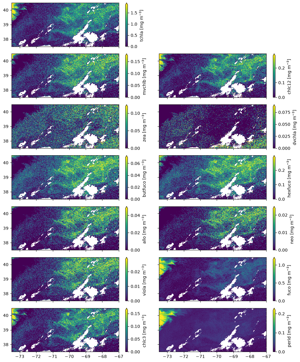
You have completed the notebook on the SDP Python algorithm!