

Merged HARP2 L2 V4.0 aerosol over ocean and land product (FastMAPOL)#
Authors: Meng Gao (NASA/SSAI), Sean Foley (NASA/MSU), Skye Caplan (NASA/SSAI)
The following notebooks are prerequisites for this tutorial:
Summary#
This notebook explores the HARP2 Level-2 (L2) aerosol products generated by FastMAPOL (Fast Multi-Angle Polarimetric Ocean and Land), a joint aerosol–surface retrieval algorithm. For more detailed information about the algorithm and data products, please refer to the FastMAPOL ATBD and associated documentation.
You should already be familiar with the aerosol-over-ocean product from the previous notebook. The current aerosol-over-ocean product generally shows better retrieval performance than the aerosol-over-land product. For aerosol product evaluation and scientific analysis, the aerosol-over-ocean product is recommended, preferably using retrievals with quality flag ≤ 1.
The aerosol-over-land product is still undergoing evaluation and should be used with caution, as the retrievals may exhibit significant biases. In this notebook, we merge the two product suites, MAPOL_OCEAN and MAPOL_LAND, to provide a convenient way to explore their similarities and differences across ocean and land.
How to Cite#
If you use the PACE HARP2 MAPOL_LAND Version 4.0 data, please refer to the dataset information page for the latest citation and DOI:
https://www.earthdata.nasa.gov/data/catalog/ob-cloud-pace-harp2-l2-mapol-land-4.0
The dataset may be cited as:
NASA Ocean Biology Processing Group. (2026). PACE HARP2 Level-2 Regional Aerosol Over LAND Optical Properties, FastMAPOL Algorithm, Version 4.0. NASA Ocean Biology Distributed Active Archive Center (OB.DAAC). DOI: 10.5067/PACE/HARP2/L2/MAPOL_LAND/4.0. Accessed on: YYYY-MM-DD.
Learning Objectives#
By the end of this notebook, you will understand:
How to acquire HARP2 L2 MAPOL_OCEAN and MAPOL_LAND data
How to merge the two data suites together
How to visualize basic aerosol properties
How to evaluate data quality
1. Setup#
Begin by importing all of the packages used in this notebook. If your kernel uses an environment defined following the guidance on the tutorials page, then the imports will be successful.
#import requests
import earthaccess
import numpy as np
import xarray as xr
#from pathlib import Path
import warnings
warnings.filterwarnings('ignore')

import matplotlib.pyplot as plt
from matplotlib.colors import LogNorm
from matplotlib.patches import Ellipse
import matplotlib.patheffects as path_effects
import cartopy.crs as ccrs
import cartopy.feature as cfeature
auth = earthaccess.login(persist=True)
fs = earthaccess.get_fsspec_https_session()
2. Get Level-2 Data#
HARP2 L2 data is available from both the Ocean Biology Distributed Active Archive Center (OB.DAAC) and NASA Earthdata. The following block retrieves a single HARP2 L2 granule at the time stamp 2025/01/09 20:00:19 UTC from both the MAPOL_LAND and MAPOL_OCEAN data suites. The most recent HARP2 data version, Version 4.0 (V4.0), is specified in the search.
temporal = (
    "2025-01-09T20:00:20",
    "2025-01-09T20:00:21",
)

results_land = earthaccess.search_data(
    short_name="PACE_HARP2_L2_MAPOL_LAND",
    temporal=temporal,
    granule_name="*V4_0*",
    count=1,
)

results_ocean = earthaccess.search_data(
    short_name="PACE_HARP2_L2_MAPOL_OCEAN",
    temporal=temporal,
    granule_name="*V4_0*",
    count=1,
)

if not results_land:
    raise FileNotFoundError("No MAPOL_LAND granule was found.")

if not results_ocean:
    raise FileNotFoundError("No MAPOL_OCEAN granule was found.")
The following cell will assess whether the data we are using cloud resources located in the same region to access the data we just found, or whether we should download that data locally. You can change the local download path as necessary.
if earthaccess.__store__.in_region:
    paths_land = earthaccess.open(results_land)
    paths_ocean = earthaccess.open(results_ocean)
else:
    paths_land = earthaccess.download(results_land, local_path="./")
    paths_ocean = earthaccess.download(results_ocean, local_path="./")
Although we just downloaded two separate HARP2 datasets covering the land and the ocean, we can merge them to create one continuous aerosol field and make working with the data easier. The next cell reads in the two separate data files and combines them with dataset_land.combine_first(). That call uses land values first, and fills any gaps with values from the ocean product where available.
datatree_land = xr.open_datatree(paths_land[0])
datatree_ocean = xr.open_datatree(paths_ocean[0])

dataset_land = xr.merge(
    datatree_land.to_dict().values(),
    compat="override",
)

dataset_ocean = xr.merge(
    datatree_ocean.to_dict().values(),
    compat="override",
)

dataset = dataset_land.combine_first(dataset_ocean)
3. Understanding HARP2 L2 product structure#
In the print out of the dataset in the next cell, we can see that the L2 HARP2 FastMAPOL product suite includes a long list (70 variables!) of data:
The MAPOL_OCEAN suite provides aquatic variables:
Wind speed (wind_speed)
Chlorophyll-a (chla)
Multi-angle and nadir Remote sensing reflectance (Rrs*)
The MAPOL_LAND suite provides terrestrial information:
Multi-angle and nadir corrected land surface reflectance (rhos*)
BRDF model parameters (Ross-Li model)
Tutorials on land surface reflectance can be found in the HARP2 Land Product notebook.
Since we merge the MAPOL_OCEAN and MAPOL_LAND suites, we can explore continuous aerosol retrievals across both ocean and land, regardless of the underlying surface type. Please refer to the HARP2 Aerosol-over-Ocean notebook for a list of available aerosol properties, or explore the dataset directly to see the available variables.
dataset
<xarray.Dataset> Size: 559MB
Dimensions:                (number_of_lines: 395, pixels_per_line: 519,
                            wavelength: 4, number_of_views: 90,
                            intensity_bands_per_view: 1,
                            polarization_bands_per_view: 1)
Coordinates:
  * wavelength             (wavelength) float32 16B 440.2 549.5 664.6 865.3
Dimensions without coordinates: number_of_lines, pixels_per_line,
                                number_of_views, intensity_bands_per_view,
                                polarization_bands_per_view
Data variables: (12/70)
    latitude               (number_of_lines, pixels_per_line) float32 820kB 1...
    longitude              (number_of_lines, pixels_per_line) float32 820kB -...
    alh                    (number_of_lines, pixels_per_line) float32 820kB n...
    vd_mode1               (number_of_lines, pixels_per_line) float32 820kB n...
    vd_mode2               (number_of_lines, pixels_per_line) float32 820kB n...
    vd_mode3               (number_of_lines, pixels_per_line) float32 820kB n...
    ...                     ...
    Rrs_angular_mean       (number_of_lines, pixels_per_line, wavelength) float32 3MB ...
    Rrs_angular_std        (number_of_lines, pixels_per_line, wavelength) float32 3MB ...
    Rrs_nadir_mean         (number_of_lines, pixels_per_line, wavelength) float32 3MB ...
    Rrs_nadir_std          (number_of_lines, pixels_per_line, wavelength) float32 3MB ...
    Rrs_angular            (number_of_lines, pixels_per_line, number_of_views, intensity_bands_per_view) float32 74MB ...
    Rrs_nadir              (number_of_lines, pixels_per_line, number_of_views, intensity_bands_per_view) float32 74MB ...
Attributes: (12/38)
    title:                  PACE HARP2 Level-2 aerosol and land product
    platform:               PACE
    instrument:             HARP2
    startDirection:         Ascending
    endDirection:           Ascending
    product_name:           PACE_HARP2.20250109T200019.L2.MAPOL_LAND.V4_0.nc
    ...                     ...
    time_coverage_start:    2025-01-09T20:00:19Z
    time_coverage_end:      2025-01-09T20:05:19Z
    reference:              https://doi.org/10.5194/amt-16-5863-2023
    comments:
    sun_earth_distance:     0.9833925
day_night_flag: DayIt should be noted that the due to the use of xr.merge(), the original netCDF groupings (e.g., geophysical_data, etc.) are no longer present, and each data variable is located in the root group.
4. Visulize HARP2 L2 aerosol properties#
Now that we know what data we have, we can start working with it. In this example, we visualize the aerosol properties for a scene observed during the LA wild fires, which occured in early 2025. The scene has both smoke and dust events, which show HARP2’s aerosol capabilities well. We read the total aerosol optical depth, single scattering albedo, and fine mode volume fraction as below:
aot = dataset["aot"].values
ssa = dataset["ssa"].values
fvf = dataset["fvf"].values
aot.shape, ssa.shape, fvf.shape
((395, 519, 4), (395, 519, 4), (395, 519))
We also need the spatial and angular dimensions as below:
lat = dataset["latitude"].values
lon = dataset["longitude"].values
plot_range = [lon.min(), lon.max(), lat.min(), lat.max()]
wavelength = dataset["wavelength"].values
print(wavelength)
[440.159 549.465 664.564 865.283]
Next, we define a function that will take in all of this information and allow us to plot any variables of interest easily.
def plot_l2_product(
    lon, lat, data,
    plot_range, label, title,
    vmin=None, vmax=None,
    figsize=(12, 4),
    ellipses=[],
    cmap="viridis",
    log_scale=False,
    land_color="#f2efe9",
    ocean_color="#dbe9f6",
):
    """Make map + histogram with optional log color scaling and land/ocean background.

    Notes:
      - Assumes lon/lat are 2D or 1D arrays available in the outer scope
        (or change signature to pass them in).
      - For log_scale=True, only positive values are used for autoscaling and histogram.
    """

    # ------------------
    # Determine vmin / vmax if not given
    # ------------------
    valid = data[np.isfinite(data)]
    if valid.size == 0:
        raise ValueError("No finite values in `data`.")

    if log_scale:
        valid = valid[valid > 0]
        if valid.size == 0:
            raise ValueError("log_scale=True but `data` has no positive finite values.")

        if vmin is None:
            vmin = np.percentile(valid, 2)
        if vmax is None:
            vmax = np.percentile(valid, 98)

        # Safety: avoid invalid/degenerate bounds
        if (vmin is None) or (vmax is None) or (vmin <= 0) or (vmin >= vmax):
            vmin = float(np.min(valid))
            vmax = float(np.max(valid))

    else:
        if vmin is None:
            vmin = np.percentile(valid, 2)
        if vmax is None:
            vmax = np.percentile(valid, 98)

        if (vmin is None) or (vmax is None) or (vmin >= vmax):
            vmin = float(np.min(valid))
            vmax = float(np.max(valid))

    # ------------------
    # Figure layout
    # ------------------
    fig = plt.figure(figsize=figsize)
    gs = fig.add_gridspec(1, 2, width_ratios=[3, 1], wspace=0.3)

    # ------------------
    # Map subplot
    # ------------------
    ax_map = fig.add_subplot(gs[0], projection=ccrs.PlateCarree())
    ax_map.set_extent(plot_range, crs=ccrs.PlateCarree())

    # Land / ocean background (behind data)
    ax_map.add_feature(cfeature.OCEAN, facecolor=ocean_color, zorder=0)
    ax_map.add_feature(cfeature.LAND, facecolor=land_color, zorder=1)

    ax_map.coastlines(resolution="110m", color="black", linewidth=0.8)
    ax_map.gridlines(draw_labels=True)

    norm = LogNorm(vmin=vmin, vmax=vmax) if log_scale else None

    pm = ax_map.pcolormesh(
        lon, lat, data,
        norm=norm,
        vmin=None if log_scale else vmin,
        vmax=None if log_scale else vmax,
        transform=ccrs.PlateCarree(),
        cmap=cmap,
        zorder=2
    )

    cbar = plt.colorbar(pm, ax=ax_map, orientation="vertical", pad=0.1)
    cbar.set_label(label)

    ax_map.set_title(title, fontsize=12)

    # ------------------
    # Histogram subplot
    # ------------------
    ax_hist = fig.add_subplot(gs[1])

    hist_data = data[np.isfinite(data)]
    if log_scale:
        hist_data = hist_data[hist_data > 0]
        bins = np.logspace(np.log10(vmin), np.log10(vmax), 40)
        ax_hist.hist(hist_data, bins=bins, color="gray", edgecolor="black")
        ax_hist.set_xscale("log")
    else:
        ax_hist.hist(
            hist_data, bins=40, range=[vmin, vmax],
            color="gray", edgecolor="black"
        )

    ax_hist.set_xlabel(label)
    ax_hist.set_ylabel("Count")
    ax_hist.set_title(f"Histogram: N={hist_data.size}")
    for ellipse in ellipses:
        ell = ax_map.add_patch(Ellipse(facecolor=(0, 0, 0, 0), lw=2, zorder=3, linestyle="dashed", **ellipse))
        ell.set_path_effects([path_effects.Stroke(linewidth=4, foreground='white'), path_effects.Normal()])
    ax_map.legend(loc="upper right")

    plt.show()
First, let’s take a look at the aerosol optical depth:
wavelength_index = 1
title = "Aerosol Optical Depth (AOD): " + str(wavelength[wavelength_index]) + " nm"
label = "AOD"
data = aot[:, :, wavelength_index]
ellipses = [
    {"label": "Smoke", "xy": (-118.5, 31), "width": 3, "height": 8, "angle": 0, "edgecolor": (0.004, 0.451, 0.698)},
    {"label": "Dust", "xy": (-113.5, 24), "width": 10, "height": 11, "angle": 15, "edgecolor": (0.871, 0.561, 0.02)},
]
plot_l2_product(
    lon, lat, data, plot_range=plot_range, label=label, title=title, vmin=0, vmax=0.3, ellipses=ellipses, cmap="YlOrRd"
)
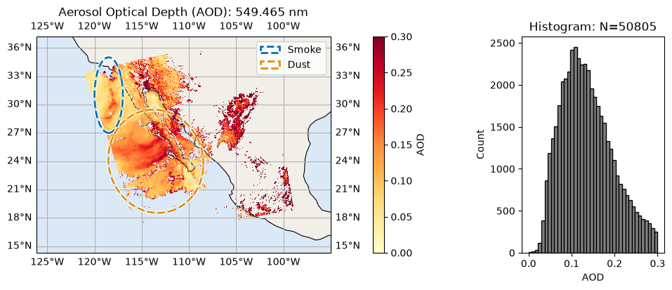
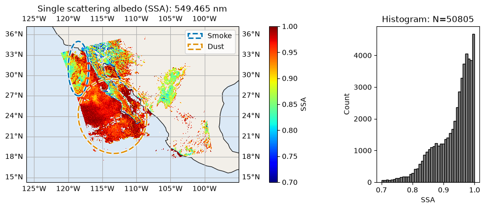
From the plot above, we can identify two regions with high AOD that might be worth a closer look. We can use the single scattering albedo (SSA) and fine mode volume fraction (FVF) to further investigate what these events might be:
wavelength_index = 1
title = "Single scattering albedo (SSA): " + str(wavelength[wavelength_index]) + " nm"
label = "SSA"
data = ssa[:, :, wavelength_index]
plot_l2_product(
    lon, lat, data, plot_range=plot_range, label=label, title=title, vmin=0.7, vmax=1, ellipses=ellipses, cmap="jet"
)
wavelength_index = 1
title = "Fine mode fraction"
label = "FVF"
data = fvf
plot_l2_product(
    lon, lat, data, plot_range=plot_range, label=label, title=title, vmin=0, vmax=1, ellipses=ellipses, cmap="jet"
)
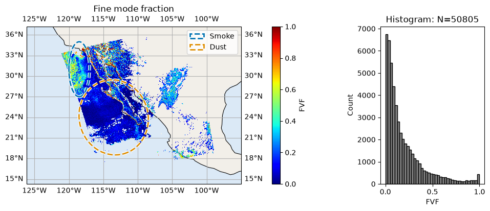
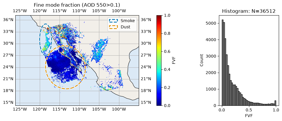
These events give off oppsosite signals in both SSA and FVF, signifying that they are likely due to different types of aerosols and thus have different origins. We can be more sure of this by zeroing in on the high quality pixels present in these maps.
5. Improving data quality: filter low AOD pixels#
Aerosol absorption and microphysics have larger uncertainties when aerosol loading is low. Users can further remove low AOD cases when necessary. With these cases removed, we can more clearly see two types of aerosol events with relatively high AOD, the upper one with high absorption (low SSA) and small size (high FVF), probably smoke due to the LA wildfires. The lower event with less absorption (high SSA) and large size (low FVF) is probably dust from off the coast of Baja California.
wavelength_index = 1
aot_min = 0.1
title = (
    "Filtered single scattering albedo (SSA): "
    + str(wavelength[wavelength_index])
    + " nm (AOD 550>"
    + str(aot_min)
    + ")"
)
label = "SSA"
data = filtered_ssa = np.where(
    aot[:, :, wavelength_index] >= aot_min, ssa[:, :, wavelength_index], np.nan
)
plot_l2_product(
    lon, lat,data, plot_range=plot_range, label=label, title=title, vmin=0.7, vmax=1, ellipses=ellipses, cmap="jet"
)
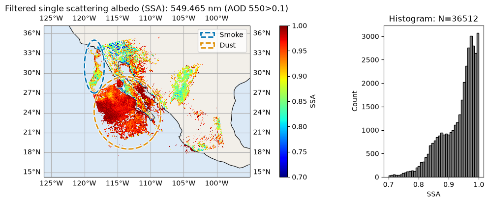
The difference in appearance (after matplotlib automatically normalizes the data) is negligible, but the difference in the physical meaning of the array values is quite important.
wavelength_index = 1
aot_min = 0.1
title = "Fine mode fraction (AOD 550>" + str(aot_min) + ")"
label = "FVF"
data = filtered_ssa = np.where(aot[:, :, wavelength_index] >= aot_min, fvf, np.nan)
plot_l2_product(
    lon, lat,data, plot_range=plot_range, label=label, title=title, vmin=0, vmax=1, ellipses=ellipses, cmap="jet"
)
6. Advanced quality assessment#
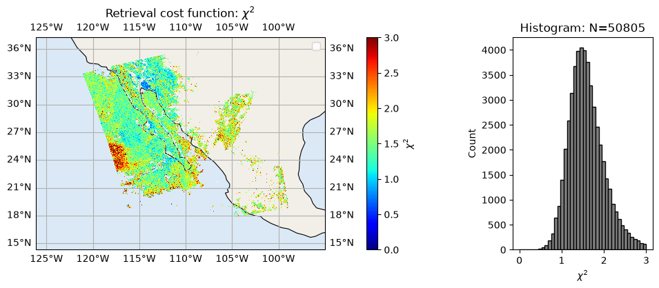
The FastMAPOL algorithm is based on optimal estimation, minimizing a \(\chi^2\) cost function defined as the difference between measurement (m) and forward model fitting (f), normalized by total uncertainties (\(\sigma\)).
\(\chi^2 = \frac{1}{N} \sum (f - m)^2/\sigma^2\)
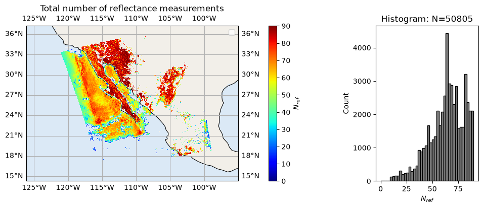
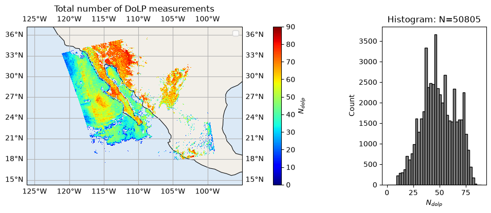
Here N is the total number of measureents used in retreival. The algorithm also adaptively evaluates fitting performance - if the fitting perform poorly, it will be removed from the retreival process. Therefore, the \(\chi^2\) and \(N\) can be used to evaluate retrieval performance. Pixels with small \(\chi^2\) (good fit) and large \(N\) (more pixels that can be fit) will better quality. A more quantitative approach based on error propogation can be also used to compute retrieval uncertainty, which will be included in future product.
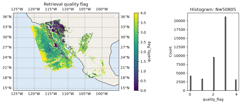
To support Level-3 data processing, quality flags are defined to indicate retrieval quality. A quality flag of 0 represents the highest-quality retrievals, generally associated with lower \(\chi^2\) and a larger number of valid measurements (\(N_v\)). Higher quality-flag values correspond to less stringent criteria, allowing larger \(\chi^2\) and fewer valid measurements. For details, please refer to the FastMAPOL ATBD Quality Flag section.
We can plot \(\chi^2\) and \(N_v\) to assess the quality of the retrievals examined in Section 5.
chi2 = dataset["chi2"].values
nv_ref = dataset["nv_ref"].values
nv_dolp = dataset["nv_dolp"].values
quality_flag = dataset["quality_flag"].values
title = r"Retrieval cost function: $\chi^2$"
label = r"$\chi^2$"
data = chi2
plot_l2_product(
    lon, lat,data, plot_range=plot_range, label=label, title=title, vmin=0, vmax=3, cmap="jet"
)
title = r"Total number of reflectance measurements"
label = r"$N_{ref}$"
data = nv_ref
plot_l2_product(
    lon, lat, data, plot_range=plot_range, label=label, title=title, vmin=0, vmax=90, cmap="jet"
)
title = r"Total number of DoLP measurements"
label = r"$N_{dolp}$"
data = nv_dolp
plot_l2_product(
    lon, lat, data, plot_range=plot_range, label=label, title=title, vmin=0, vmax=90, cmap="jet"
)
We can also take a look at the averages of these quality indicators, to get a sense of the whole scene:
np.nanmean(chi2), np.nanmean(nv_ref), np.nanmean(nv_dolp)
(np.float32(1.601495),
 np.float64(63.89646688318079),
 np.float64(48.909457730538335))
Note that \(\chi^2\) converges reasonably well with slight under fitting (an average around 1.6 and peak around 1.3). Since HARP2 measures 90 angles across 4 bands, the average number of measurements satisfying a good fit is only 52 for reflectance and 42 for DoLP, which indicates a potential discrepancy between the forward model and measurements. This is likely due to forward model assumptions or measurement calibrations.
Now that we know what is behind the quality flagging, let’s see how that informs the overall quality flag by variable:
title = "Retrieval quality flag"
label = "quality_flag"
data = quality_flag
plot_l2_product(
    lon, lat, data, plot_range=plot_range, label=label, title=title, vmin=0, vmax=4, cmap="viridis"
)
7. Multi-angle data mask for cloud and data screening#
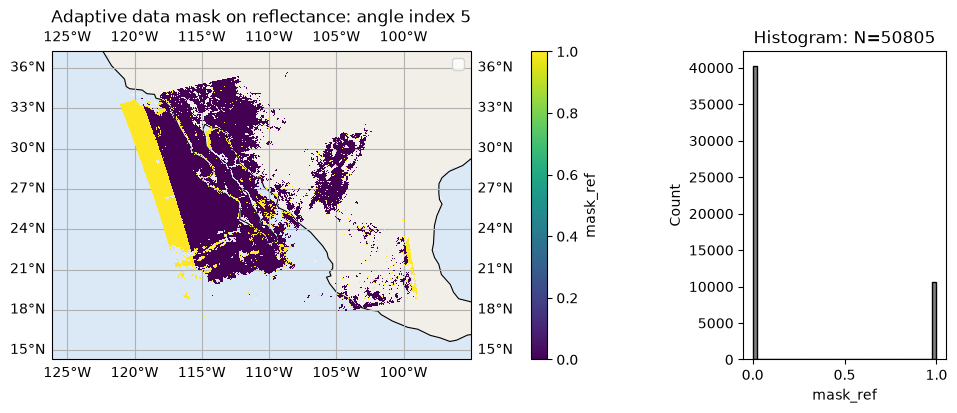
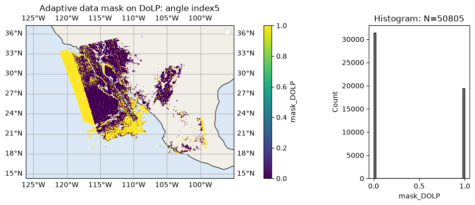
As mentioned previously, the FastMAPOL algorithm conducts internal adaptive data screening on each HARP2 angle. The data masks are provided for both reflectance and DoLP. A value of 0 means the measurements are used in the retrievals, while a value of 1 or nan means the measurements were removed from the retrieval. Therefore, the adaptive data mask can be also used to evaluate fitting quality and measurement quality at each angle. In the example below, please note the different pattern for reflectance and polarization, which may indicate different calibration performance.
mask_ref = dataset["mask_ref"].values
mask_dolp = dataset["mask_dolp"].values
mask_ref.shape, mask_dolp.shape
((395, 519, 90, 1), (395, 519, 90, 1))
angle_index = 5
title = "Adaptive data mask on reflectance: angle index " + str(angle_index)
label = "mask_ref"
data = mask_ref[:, :, angle_index, 0]
plot_l2_product(
    lon, lat, data, plot_range=plot_range, label=label, title=title, vmin=0, vmax=1, cmap="viridis"
)
angle_index = 5
title = "Adaptive data mask on DoLP: angle index" + str(angle_index)
label = "mask_DOLP"
data = mask_dolp[:, :, angle_index, 0]
plot_l2_product(
    lon, lat, data, plot_range=plot_range, label=label, title=title, vmin=0, vmax=1, cmap="viridis"
)
8. Optional: pixel level uncertainty estimation.#
As mentioned previously, pixel level uncertainty can be evalated through error propagation, which propagate measurement uncertainty through the Jacobian of the forward model. The estimated uncertainties are discussed in (Gao et al., 2021) for HARP2 and AirHARP, but are currently not included in the HARP2 L2 products.
9. Reference#
[Validation] Gao, M., Aryal, K., Zhai, P.-W., Knobelspiesse, K., Franz, B. A., Cairns, B., Cetinić, I., Fu, G., Hasekamp, O., Ibrahim, A., Sayer, A. M., and Werdell, P. J.: Where sky meets sea: Integrated aerosol and ocean color retrieval from PACE SPEXone multi-angle polarimetry, Remote Sens. Environ., 345, 115603, https://doi.org/10.1016/j.rse.2026.115603, 2026.
[Algorithm] Gao, M., Franz, B. A., Zhai, P.-W., Knobelspiesse, K., Sayer, A. M., Xu, X., Martins, J. V., Cairns, B., Castellanos, P., Fu, G., Hannadige, N., Hasekamp, O., Hu, Y., Ibrahim, A., Patt, F., Puthukkudy, A., and Werdell, P. J.: Simultaneous retrieval of aerosol and ocean properties from PACE HARP2 with uncertainty assessment using cascading neural network radiative transfer models, Atmos. Meas. Tech., 16, 5863–5881, https://doi.org/10.5194/amt-16-5863-2023, 2023.