Demo: Fault Simulation and Analysis

This notebook shows basic I/O operations that can be performed with fmdtools, as well as some of the basic model and simulation visualization and analysis features.

This is helpful for understanding the breadth of fmdtools plotting, tabulation, and visualization capabilities. Specifically, it covers:

• A variety of graphing use-cases in graph functions which enable viewing different graph types, simulation results at individual times, and overall model statistics/results.

• tabulate functions for viewing simulation results over time and summarizing run information.

• Saving/Loading Result data structures.

This script runs these basic operations on the simple model defined in model_main.py.

Copyright © 2024, United States Government, as represented by the Administrator of the National Aeronautics and Space Administration. All rights reserved.

The “"Fault Model Design tools - fmdtools version 2"” software is licensed under the Apache License, Version 2.0 (the "License"); you may not use this file except in compliance with the License. You may obtain a copy of the License at http://www.apache.org/licenses/LICENSE-2.0. 

Unless required by applicable law or agreed to in writing, software distributed under the License is distributed on an "AS IS" BASIS, WITHOUT WARRANTIES OR CONDITIONS OF ANY KIND, either express or implied. See the License for the specific language governing permissions and limitations under the License.

from model_main import Pump

import fmdtools.sim.propagate as propagate
from fmdtools import analyze as an

from IPython.display import HTML

Initial Model Checks

Before seeing how faults propagate, it’s useful to see that the model structure is set up correctly and that the system performs as expected.

The ‘track’ argument specifies what model attributes to log. Specifying all will log all attributes.

mdl = Pump(track='all')

One of the easiest ways to visualize this is by viewing the model in the repl, which shows thes states and modes of the component functions and flows.

mdl

pump Pump
- t=Time(time=-0.1, timers={})
- m=Mode(mode='nominal', faults=set(), sub_faults=False)
FLOWS:
- ee_1=Electricity(s=(current=1.0, voltage=1.0))
- sig_1=Signal(s=(power=1.0))
- wat_1=Water(s=(flowrate=1.0, pressure=1.0, area=1.0, level=1.0))
- wat_2=Water(s=(flowrate=1.0, pressure=1.0, area=1.0, level=1.0))
FXNS:
- import_ee=ImportEE(s=(effstate=1.0), m=(mode='nominal', faults=set(), sub_faults=False))
- import_water=ImportWater(m=(mode='nominal', faults=set(), sub_faults=False))
- import_signal=ImportSig(m=(mode='nominal', faults=set(), sub_faults=False))
- move_water=MoveWat(s=(eff=1.0), m=(mode='nominal', faults=set(), sub_faults=False))
- export_water=ExportWater(m=(mode='nominal', faults=set(), sub_faults=False))

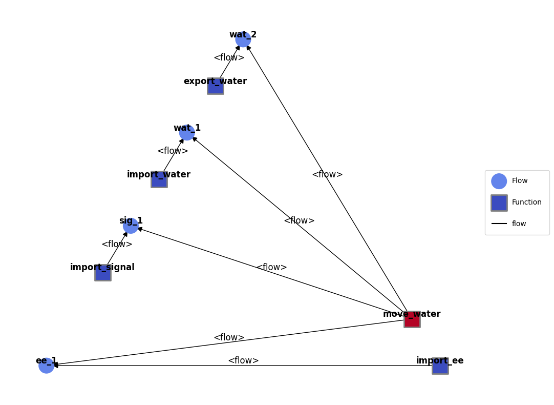
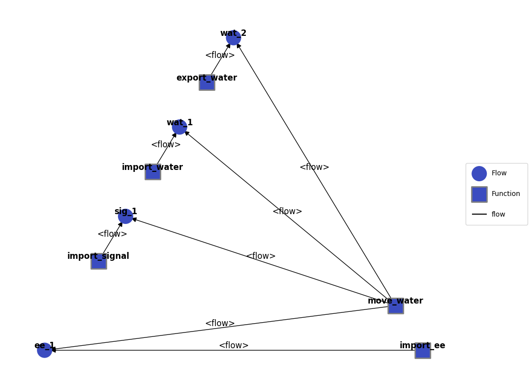
Model Structure Visualization

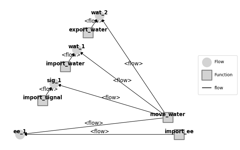
To check that the simulation structures are set up right, the FunctionArchitectureGraph class lets us visualize the function/flow relationships in the model. This helps us answer the questions:

• are all functions on the graph?

• are the functions connected with the correct flows?

from fmdtools.define.architecture.function import FunctionArchitectureGraph

a = FunctionArchitectureGraph(mdl)
fig, ax = a.draw(figsize=(8,6))

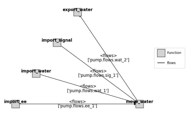
Note that a variety of different Classes can be used for model structure visualization, inlcluding ModelFxnGraph, ModelFlowGraph, and ModelTypeGraph. This is further explained in examples/navigating_rover/Model_Structure_Visualization_Tutorial.ipynb

from fmdtools.define.architecture.function import FunctionArchitectureFxnGraph
b=FunctionArchitectureFxnGraph(mdl)
fig = b.draw(figsize=(8,6))

Nominal Run

The next code runs the model in the nominal state to check to see that the model has been defined correctly. This helps us verify:

• if any faults occur in the nominal scenario

• if the progression of states proceeds as desired over time.

The following code runs the model with no faults to let us do that. The inputs are:

• mdl (the model we imported at the start of the script)

• to_return (str/list/dict describing what to return in result)

• **kwargs (see docs)

The outputs are:

• result (a Result object defined in analyze.result)

• mdlhist (a History object defined in analyze.result)

Both Result and History have a number of methods that can be readily used to process and analyze simulation results. See:

• Result documentation

• History documentation

Many different properties can be requested given the to_return argument (see full list here). In this case, we pass a dict with key graph and a value FunctionArchitectureGraph specifying that we want it to give us a graph view of the Model.

result, mdlhist = propagate.nominal(mdl, to_return={'graph': FunctionArchitectureGraph})

Here we can see where it is in the Result:

result.keys()

dict_keys(['tend.graph'])

graph = result.tend.graph

With these results, we can now plot the graph of results resgraph using:

fig = graph.draw(figsize=(6,4))

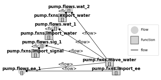
As can be seen, this gives a graphical representation of the functional model with the various flows. Since all of the functions are grey, no faults were accidentally introduced in this run.

A model history is additionally returned given our specified tracking options. If none are provided, the default_track variable in the Model is used (which in this case is set to all). See below:

mdlhist

i.finished:                    array(56)
i.on:                          array(56)
m.sub_faults:                  array(56)
time:                          array(56)
flows.ee_1.s.current:          array(56)
flows.ee_1.s.voltage:          array(56)
flows.sig_1.s.power:           array(56)
flows.wat_1.s.flowrate:        array(56)
flows.wat_1.s.pressure:        array(56)
flows.wat_1.s.area:            array(56)
flows.wat_1.s.level:           array(56)
flows.wat_2.s.flowrate:        array(56)
flows.wat_2.s.pressure:        array(56)
flows.wat_2.s.area:            array(56)
flows.wat_2.s.level:           array(56)
fxns.import_ee.s.effstate:     array(56)
fxns.import_ee.m.faults.inf_v: array(56)
fxns.import_ee.m.faults.no_v:  array(56)
fxns.import_ee.m.sub_faults:   array(56)
fxns.import_water.m.faults.less_wat: array(56)
fxns.import_water.m.faults.no_wat: array(56)
fxns.import_water.m.sub_faults: array(56)
fxns.import_signal.m.faults.no_sig: array(56)
fxns.import_signal.m.sub_faults: array(56)
fxns.move_water.i.over_pressure: array(56)
fxns.move_water.s.eff:         array(56)
fxns.move_water.m.faults.mech_break: array(56)
fxns.move_water.m.faults.short: array(56)
fxns.move_water.m.sub_faults:  array(56)
fxns.move_water.t.pressure_limit.time: array(56)
fxns.move_water.t.pressure_limit.mode: array(56)
fxns.export_water.m.faults.block: array(56)
fxns.export_water.m.sub_faults: array(56)

We can further look at the states of the model over time using History.plot_line:

fig, ax = mdlhist.plot_line('flows.wat_1.s.flowrate', 'flows.wat_2.s.flowrate', 'i.on', 'flows.sig_1.s.power')

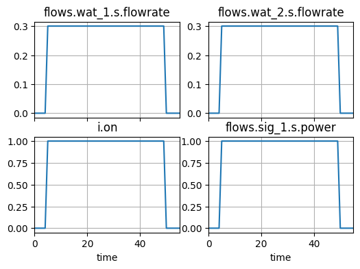
As we can see, the state of these flows does exactly what we would expect–when the switch turns on at $t=5$, the pump switches on and there is a flow of water in and out of the model.

History

If we want to see this data in tabular form, we can use fp.tabulate.hist():

nominal_histtable = mdlhist.as_table()
nominal_histtable[:10] #only displaying 10 

	i.finished	i.on	m.sub_faults	time	flows.ee_1.s.current	...	fxns.move_water.m.sub_faults	fxns.move_water.t.pressure_limit.time	fxns.move_water.t.pressure_limit.mode	fxns.export_water.m.faults.block	fxns.export_water.m.sub_faults
0	False	False	False	0.0	0.0	...	False	0.0	standby	False	False
1	False	False	False	1.0	0.0	...	False	0.0	standby	False	False
2	False	False	False	2.0	0.0	...	False	0.0	standby	False	False
3	False	False	False	3.0	0.0	...	False	0.0	standby	False	False
4	False	False	False	4.0	0.0	...	False	0.0	standby	False	False
5	False	True	False	5.0	10.0	...	False	0.0	standby	False	False
6	False	True	False	6.0	10.0	...	False	0.0	standby	False	False
7	False	True	False	7.0	10.0	...	False	0.0	standby	False	False
8	False	True	False	8.0	10.0	...	False	0.0	standby	False	False
9	False	True	False	9.0	10.0	...	False	0.0	standby	False	False

10 rows × 33 columns

This table is a pandas dataframe. We can save this dataframe to a .csv using nominal_histtable.to_csv("filename.csv")

Propagating and Viewing Results for Individual Faults

It is often necessary to see how the system reacts to individual faults. This can gives us better understanding of how the system behaves under individual faults and can let us iterate with the model better.

The following code runs the model with a single fault in a single function. In this case, we are initiating a short in the ‘Move Water’ function at 10 hours into the system’s operation.

The inputs are:

• mdl (the model we imported at the start of the script)

• function (the function the fault we’re interested in propagating occurs in)

• faultmode (the fault to initiate)

• time (the time when the fault is initiated)

• **kwargs )

The outputs are (the same as propogate.nominal):

• results (a dictionary corresponding to to_return)

• mdlhist (the states of the model over time)

endresults, mdlhist=propagate.one_fault(mdl, 'move_water', 'short', time=10, 
                                        to_return=['graph','classify','endfaults'])

Now mdlhist has double the number of entries–those corresponding to the nominal and faulty scenarios.

mdlhist

nominal.i.finished:            array(56)
nominal.i.on:                  array(56)
nominal.m.sub_faults:          array(56)
nominal.time:                  array(56)
nominal.flows.ee_1.s.current:  array(56)
nominal.flows.ee_1.s.voltage:  array(56)
nominal.flows.sig_1.s.power:   array(56)
nominal.flows.wat_1.s.flowrate: array(56)
nominal.flows.wat_1.s.pressure: array(56)
nominal.flows.wat_1.s.area:    array(56)
nominal.flows.wat_1.s.level:   array(56)
nominal.flows.wat_2.s.flowrate: array(56)
nominal.flows.wat_2.s.pressure: array(56)
nominal.flows.wat_2.s.area:    array(56)
nominal.flows.wat_2.s.level:   array(56)
nominal.fxns.import_ee.s.effstate: array(56)
nominal.fxns.import_ee.m.faults.inf_v: array(56)
nominal.fxns.import_ee.m.faults.no_v: array(56)
nominal.fxns.import_ee.m.sub_faults: array(56)
nominal.fxns.import_           array(56)
nominal.fxns.import_           array(56)
nominal.fxns.import_water.m.sub_faults: array(56)
nominal.fxns.import_           array(56)
nominal.fxns.import_           array(56)
nominal.fxns.move_wa           array(56)
nominal.fxns.move_water.s.eff: array(56)
nominal.fxns.move_wa           array(56)
nominal.fxns.move_water.m.faults.short: array(56)
nominal.fxns.move_water.m.sub_faults: array(56)
nominal.fxns.move_wa           array(56)
nominal.fxns.move_wa           array(56)
nominal.fxns.export_           array(56)
nominal.fxns.export_water.m.sub_faults: array(56)
move_water_short_t10.i.finished: array(56)
move_water_short_t10.i.on:     array(56)
move_water_short_t10.m.sub_faults: array(56)
move_water_short_t10.time:     array(56)
move_water_short_t10           array(56)
move_water_short_t10           array(56)
move_water_short_t10           array(56)
move_water_short_t10           array(56)
move_water_short_t10           array(56)
move_water_short_t10           array(56)
move_water_short_t10           array(56)
move_water_short_t10           array(56)
move_water_short_t10           array(56)
move_water_short_t10           array(56)
move_water_short_t10           array(56)
move_water_short_t10           array(56)
move_water_short_t10           array(56)
move_water_short_t10           array(56)
move_water_short_t10           array(56)
move_water_short_t10           array(56)
move_water_short_t10           array(56)
move_water_short_t10           array(56)
move_water_short_t10           array(56)
move_water_short_t10           array(56)
move_water_short_t10           array(56)
move_water_short_t10           array(56)
move_water_short_t10           array(56)
move_water_short_t10           array(56)
move_water_short_t10           array(56)
move_water_short_t10           array(56)
move_water_short_t10           array(56)
move_water_short_t10           array(56)
move_water_short_t10           array(56)

History.get_degraded_hist compares the results over time so we can see what functions and flows were degraded over time. We can then use the summary to view a list of the functions and flows that were impacted over time.

deghist = mdlhist.get_degraded_hist(*mdl.fxns, *mdl.flows)

deghist

import_ee:                     array(56)
import_water:                  array(56)
import_signal:                 array(56)
move_water:                    array(56)
export_water:                  array(56)
ee_1:                          array(56)
sig_1:                         array(56)
wat_1:                         array(56)
wat_2:                         array(56)
total:                         array(56)
time:                          array(56)

deghist.as_table()

	import_ee	import_water	import_signal	move_water	export_water	...	sig_1	wat_1	wat_2	total	time
0	False	False	False	False	False	...	False	False	False	0	0.0
1	False	False	False	False	False	...	False	False	False	0	1.0
2	False	False	False	False	False	...	False	False	False	0	2.0
3	False	False	False	False	False	...	False	False	False	0	3.0
4	False	False	False	False	False	...	False	False	False	0	4.0
5	False	False	False	False	False	...	False	False	False	0	5.0
6	False	False	False	False	False	...	False	False	False	0	6.0
7	False	False	False	False	False	...	False	False	False	0	7.0
8	False	False	False	False	False	...	False	False	False	0	8.0
9	False	False	False	False	False	...	False	False	False	0	9.0
10	False	False	False	True	False	...	False	False	False	1	10.0
11	False	False	False	True	False	...	False	False	False	1	11.0
12	False	False	False	True	False	...	False	False	False	1	12.0
13	False	False	False	True	False	...	False	False	False	1	13.0
14	False	False	False	True	False	...	False	False	False	1	14.0
15	False	False	False	True	False	...	False	False	False	1	15.0
16	False	False	False	True	False	...	False	False	False	1	16.0
17	False	False	False	True	False	...	False	False	False	1	17.0
18	False	False	False	True	False	...	False	False	False	1	18.0
19	False	False	False	True	False	...	False	False	False	1	19.0
20	False	False	False	True	False	...	False	False	False	1	20.0
21	False	False	False	True	False	...	False	False	False	1	21.0
22	False	False	False	True	False	...	False	False	False	1	22.0
23	False	False	False	True	False	...	False	False	False	1	23.0
24	False	False	False	True	False	...	False	False	False	1	24.0
25	False	False	False	True	False	...	False	False	False	1	25.0
26	False	False	False	True	False	...	False	False	False	1	26.0
27	False	False	False	True	False	...	False	False	False	1	27.0
28	False	False	False	True	False	...	False	False	False	1	28.0
29	False	False	False	True	False	...	False	False	False	1	29.0
30	False	False	False	True	False	...	False	False	False	1	30.0
31	False	False	False	True	False	...	False	False	False	1	31.0
32	False	False	False	True	False	...	False	False	False	1	32.0
33	False	False	False	True	False	...	False	False	False	1	33.0
34	False	False	False	True	False	...	False	False	False	1	34.0
35	False	False	False	True	False	...	False	False	False	1	35.0
36	False	False	False	True	False	...	False	False	False	1	36.0
37	False	False	False	True	False	...	False	False	False	1	37.0
38	False	False	False	True	False	...	False	False	False	1	38.0
39	False	False	False	True	False	...	False	False	False	1	39.0
40	False	False	False	True	False	...	False	False	False	1	40.0
41	False	False	False	True	False	...	False	False	False	1	41.0
42	False	False	False	True	False	...	False	False	False	1	42.0
43	False	False	False	True	False	...	False	False	False	1	43.0
44	False	False	False	True	False	...	False	False	False	1	44.0
45	False	False	False	True	False	...	False	False	False	1	45.0
46	False	False	False	True	False	...	False	False	False	1	46.0
47	False	False	False	True	False	...	False	False	False	1	47.0
48	False	False	False	True	False	...	False	False	False	1	48.0
49	False	False	False	True	False	...	False	False	False	1	49.0
50	False	False	False	True	False	...	True	True	True	5	50.0
51	False	False	False	True	False	...	True	True	True	5	51.0
52	False	False	False	True	False	...	True	True	True	5	52.0
53	False	False	False	True	False	...	True	True	True	5	53.0
54	False	False	False	True	False	...	True	True	True	5	54.0
55	False	False	False	True	False	...	True	True	True	5	55.0

56 rows × 11 columns

endresults however, keeps the endresult for the faulty scenario alone, as shown:

endresults

nominal.tend.classify.rate:          1.0
nominal.tend.classify.cost:          0.0
nominal.tend.classify.expected_cost: 0.0
nominal.tend.graph: <fmdtools.define.architecture.function.FunctionArchitectureGraph object at 0x0000020453CFF110>
move_water_short_t10               1e-05
move_water_short_t10              8650.0
move_water_short_t10              8650.0
move_water_short_t10.tend.graph: <fmdtools.define.architecture.function.FunctionArchitectureGraph object at 0x00000204538C0E90>

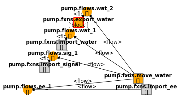
However, the graph view now has information about degradations between the faulty and nominal runs, along with fault information:

faultgraph = endresults.get_faulty().tend.graph
fig = faultgraph.draw()

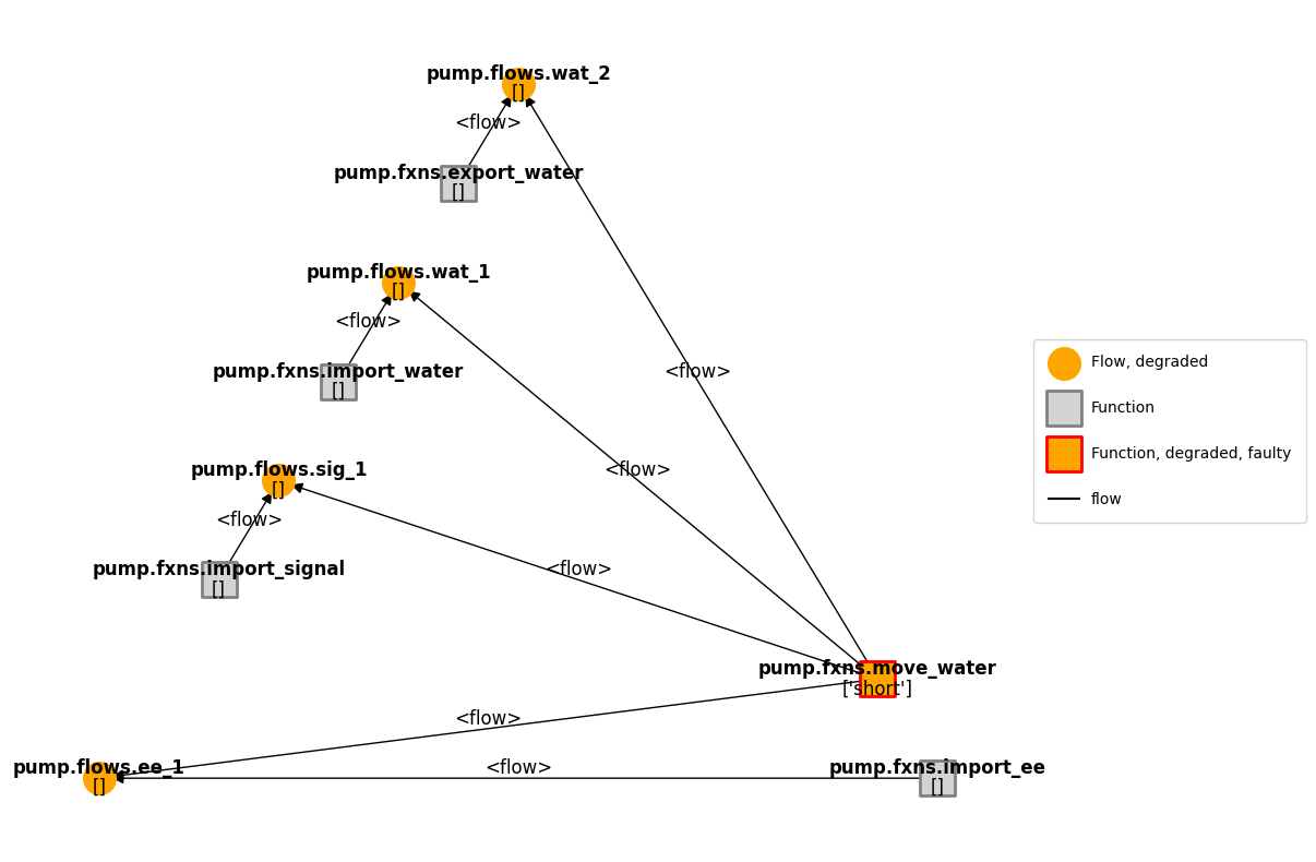
faultgraph.g.nodes['pump.fxns.move_water']

{'nodetype': 'Function',
 'classname': 'MoveWat',
 't': MoveWatTime(time=55.0, t_ind=55, timers={'pressure_limit': Timer pressure_limit: mode= standby, time= 0.0}, use_local=True, dt=1.0, executed_static=True, executed_dynamic=False, executing=False),
 's': MoveWatStates(eff=0.0),
 'm': MoveWatMode(faults={'short'}, sub_faults=False),
 'indicators': [],
 'degraded': True,
 'faulty': True}

As can be seen, at the final t, the short causes a degraded flow of electricity as well as a fault in the Import EE function.

However, we would imagine that the short would cause the water to stop moving also–so why is it not red?

The answer is that by default the degradations shown in the graph are shown at the final time, which is the same both for the failed model and the nominal model, since the pump is switched “off.” In this case we might be more interested in looking at how the graph looks in operation, rather than at the end.

We can do that that in two ways:

• by specifying a different time to fetch the graph from (e.g., to_return={10:'graph'}, or

• by reconstructing the based on the history of the plot, as shown below:

mg = FunctionArchitectureGraph(mdl)

To do this, we first need to track more states than have been specified to track in the model. The easiest way to do this is to set track='all'.

endresults, mdlhist_full=propagate.one_fault(mdl, 'move_water', 'short', time=10, track='all',
                                        to_return=['graph','classify','endfaults'])

We can then plot the state at any time in the history using mg.draw_from.

fig, ax = mg.draw_from(15, mdlhist_full)

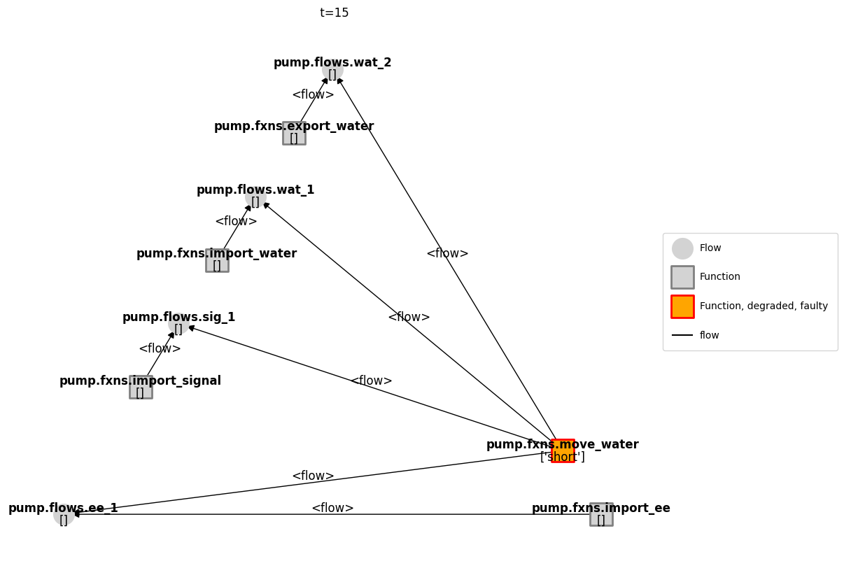
As shown, this version has the degradation of the water, since at this time the off-nominal state is different from the nominal (no flow).

We can view an animation over time using:

from IPython.display import HTML
ani = mg.animate(mdlhist_full)
HTML(ani.to_jshtml())

Once Loop Reflect

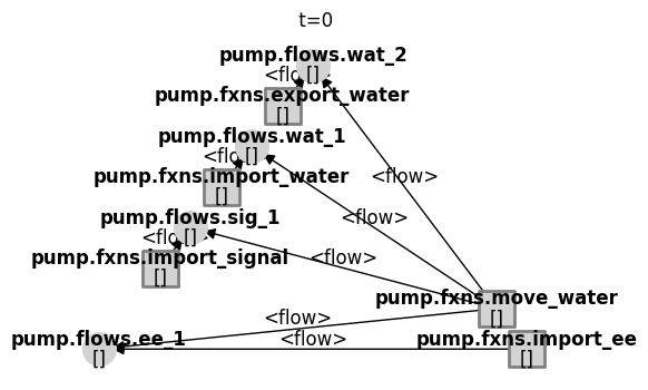
Note that if only a partial history is given, only partial results will be displayed (see below).

fig, ax = mg.draw_from(15, mdlhist, figsize=(6,4), withlegend=False)

We can also plot the states of this against the nominal run using:

mdlhist

nominal.i.finished:            array(56)
nominal.i.on:                  array(56)
nominal.m.sub_faults:          array(56)
nominal.time:                  array(56)
nominal.flows.ee_1.s.current:  array(56)
nominal.flows.ee_1.s.voltage:  array(56)
nominal.flows.sig_1.s.power:   array(56)
nominal.flows.wat_1.s.flowrate: array(56)
nominal.flows.wat_1.s.pressure: array(56)
nominal.flows.wat_1.s.area:    array(56)
nominal.flows.wat_1.s.level:   array(56)
nominal.flows.wat_2.s.flowrate: array(56)
nominal.flows.wat_2.s.pressure: array(56)
nominal.flows.wat_2.s.area:    array(56)
nominal.flows.wat_2.s.level:   array(56)
nominal.fxns.import_ee.s.effstate: array(56)
nominal.fxns.import_ee.m.faults.inf_v: array(56)
nominal.fxns.import_ee.m.faults.no_v: array(56)
nominal.fxns.import_ee.m.sub_faults: array(56)
nominal.fxns.import_           array(56)
nominal.fxns.import_           array(56)
nominal.fxns.import_water.m.sub_faults: array(56)
nominal.fxns.import_           array(56)
nominal.fxns.import_           array(56)
nominal.fxns.move_wa           array(56)
nominal.fxns.move_water.s.eff: array(56)
nominal.fxns.move_wa           array(56)
nominal.fxns.move_water.m.faults.short: array(56)
nominal.fxns.move_water.m.sub_faults: array(56)
nominal.fxns.move_wa           array(56)
nominal.fxns.move_wa           array(56)
nominal.fxns.export_           array(56)
nominal.fxns.export_water.m.sub_faults: array(56)
move_water_short_t10.i.finished: array(56)
move_water_short_t10.i.on:     array(56)
move_water_short_t10.m.sub_faults: array(56)
move_water_short_t10.time:     array(56)
move_water_short_t10           array(56)
move_water_short_t10           array(56)
move_water_short_t10           array(56)
move_water_short_t10           array(56)
move_water_short_t10           array(56)
move_water_short_t10           array(56)
move_water_short_t10           array(56)
move_water_short_t10           array(56)
move_water_short_t10           array(56)
move_water_short_t10           array(56)
move_water_short_t10           array(56)
move_water_short_t10           array(56)
move_water_short_t10           array(56)
move_water_short_t10           array(56)
move_water_short_t10           array(56)
move_water_short_t10           array(56)
move_water_short_t10           array(56)
move_water_short_t10           array(56)
move_water_short_t10           array(56)
move_water_short_t10           array(56)
move_water_short_t10           array(56)
move_water_short_t10           array(56)
move_water_short_t10           array(56)
move_water_short_t10           array(56)
move_water_short_t10           array(56)
move_water_short_t10           array(56)
move_water_short_t10           array(56)
move_water_short_t10           array(56)
move_water_short_t10           array(56)

fig, axs = mdlhist.plot_line('flows.ee_1.s.current', 'flows.wat_2.s.flowrate', 
                             title="Response of Pump to Short", time_slice=10, legend_loc=False, title_padding=0.1)

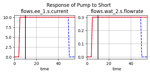
As you can see, the system begins nominal until the fault is injected at $t=10$. At this moment, not only are the electrical energy flows degraded, the flow of water is degraded also. However, at $t=55$ when the system is supposed to be turned off, this flow of water is no longer “degraded” because it is in the same state as the nominal system.

We can look at a table of to see more precisely what happened (and export, if needed). Note that we need to give the plotting function the mode (‘short’) and the time for it to plot properly.

mdlhist.as_table()

	nominal.i.finished	nominal.i.on	nominal.m.sub_faults	nominal.time	nominal.flows.ee_1.s.current	...	move_water_short_t10.fxns.move_water.m.sub_faults	move_water_short_t10.fxns.move_water.t.pressure_limit.time	move_water_short_t10.fxns.move_water.t.pressure_limit.mode	move_water_short_t10.fxns.export_water.m.faults.block	move_water_short_t10.fxns.export_water.m.sub_faults
0	False	False	False	0.0	0.0	...	False	0.0	standby	False	False
1	False	False	False	1.0	0.0	...	False	0.0	standby	False	False
2	False	False	False	2.0	0.0	...	False	0.0	standby	False	False
3	False	False	False	3.0	0.0	...	False	0.0	standby	False	False
4	False	False	False	4.0	0.0	...	False	0.0	standby	False	False
5	False	True	False	5.0	10.0	...	False	0.0	standby	False	False
6	False	True	False	6.0	10.0	...	False	0.0	standby	False	False
7	False	True	False	7.0	10.0	...	False	0.0	standby	False	False
8	False	True	False	8.0	10.0	...	False	0.0	standby	False	False
9	False	True	False	9.0	10.0	...	False	0.0	standby	False	False
10	False	True	False	10.0	10.0	...	False	0.0	standby	False	False
11	False	True	False	11.0	10.0	...	False	0.0	standby	False	False
12	False	True	False	12.0	10.0	...	False	0.0	standby	False	False
13	False	True	False	13.0	10.0	...	False	0.0	standby	False	False
14	False	True	False	14.0	10.0	...	False	0.0	standby	False	False
15	False	True	False	15.0	10.0	...	False	0.0	standby	False	False
16	False	True	False	16.0	10.0	...	False	0.0	standby	False	False
17	False	True	False	17.0	10.0	...	False	0.0	standby	False	False
18	False	True	False	18.0	10.0	...	False	0.0	standby	False	False
19	False	True	False	19.0	10.0	...	False	0.0	standby	False	False
20	False	True	False	20.0	10.0	...	False	0.0	standby	False	False
21	False	True	False	21.0	10.0	...	False	0.0	standby	False	False
22	False	True	False	22.0	10.0	...	False	0.0	standby	False	False
23	False	True	False	23.0	10.0	...	False	0.0	standby	False	False
24	False	True	False	24.0	10.0	...	False	0.0	standby	False	False
25	False	True	False	25.0	10.0	...	False	0.0	standby	False	False
26	False	True	False	26.0	10.0	...	False	0.0	standby	False	False
27	False	True	False	27.0	10.0	...	False	0.0	standby	False	False
28	False	True	False	28.0	10.0	...	False	0.0	standby	False	False
29	False	True	False	29.0	10.0	...	False	0.0	standby	False	False
30	False	True	False	30.0	10.0	...	False	0.0	standby	False	False
31	False	True	False	31.0	10.0	...	False	0.0	standby	False	False
32	False	True	False	32.0	10.0	...	False	0.0	standby	False	False
33	False	True	False	33.0	10.0	...	False	0.0	standby	False	False
34	False	True	False	34.0	10.0	...	False	0.0	standby	False	False
35	False	True	False	35.0	10.0	...	False	0.0	standby	False	False
36	False	True	False	36.0	10.0	...	False	0.0	standby	False	False
37	False	True	False	37.0	10.0	...	False	0.0	standby	False	False
38	False	True	False	38.0	10.0	...	False	0.0	standby	False	False
39	False	True	False	39.0	10.0	...	False	0.0	standby	False	False
40	False	True	False	40.0	10.0	...	False	0.0	standby	False	False
41	False	True	False	41.0	10.0	...	False	0.0	standby	False	False
42	False	True	False	42.0	10.0	...	False	0.0	standby	False	False
43	False	True	False	43.0	10.0	...	False	0.0	standby	False	False
44	False	True	False	44.0	10.0	...	False	0.0	standby	False	False
45	False	True	False	45.0	10.0	...	False	0.0	standby	False	False
46	False	True	False	46.0	10.0	...	False	0.0	standby	False	False
47	False	True	False	47.0	10.0	...	False	0.0	standby	False	False
48	False	True	False	48.0	10.0	...	False	0.0	standby	False	False
49	False	True	False	49.0	10.0	...	False	0.0	standby	False	False
50	False	False	False	50.0	0.0	...	False	0.0	standby	False	False
51	False	False	False	51.0	0.0	...	False	0.0	standby	False	False
52	False	False	False	52.0	0.0	...	False	0.0	standby	False	False
53	False	False	False	53.0	0.0	...	False	0.0	standby	False	False
54	False	False	False	54.0	0.0	...	False	0.0	standby	False	False
55	False	False	False	55.0	0.0	...	False	0.0	standby	False	False

56 rows × 66 columns

Here we can see that the short dropped the voltage to zero, (this was because an open circuit resulted in the Import EE function), causing the water to stop flowing. Below, we use the processed model history to show the faults and degradation of states over time. In this case, 1 means nominal while 0 means degraded.

deghist = mdlhist_full.get_degraded_hist(*mdl.fxns, *mdl.flows)

deghist.as_table()[:20]

	import_ee	import_water	import_signal	move_water	export_water	...	sig_1	wat_1	wat_2	total	time
0	False	False	False	False	False	...	False	False	False	0	0.0
1	False	False	False	False	False	...	False	False	False	0	1.0
2	False	False	False	False	False	...	False	False	False	0	2.0
3	False	False	False	False	False	...	False	False	False	0	3.0
4	False	False	False	False	False	...	False	False	False	0	4.0
5	False	False	False	False	False	...	False	False	False	0	5.0
6	False	False	False	False	False	...	False	False	False	0	6.0
7	False	False	False	False	False	...	False	False	False	0	7.0
8	False	False	False	False	False	...	False	False	False	0	8.0
9	False	False	False	False	False	...	False	False	False	0	9.0
10	False	False	False	True	False	...	False	False	False	1	10.0
11	False	False	False	True	False	...	False	False	False	1	11.0
12	False	False	False	True	False	...	False	False	False	1	12.0
13	False	False	False	True	False	...	False	False	False	1	13.0
14	False	False	False	True	False	...	False	False	False	1	14.0
15	False	False	False	True	False	...	False	False	False	1	15.0
16	False	False	False	True	False	...	False	False	False	1	16.0
17	False	False	False	True	False	...	False	False	False	1	17.0
18	False	False	False	True	False	...	False	False	False	1	18.0
19	False	False	False	True	False	...	False	False	False	1	19.0

20 rows × 11 columns

We can also look at the faults over time…

faulthist = mdlhist_full.get_faulty_hist(*mdl.fxns)
faulthist.as_table()[0:20]

	import_ee	import_water	import_signal	move_water	export_water	total	time
0	False	False	False	False	False	0	0.0
1	False	False	False	False	False	0	1.0
2	False	False	False	False	False	0	2.0
3	False	False	False	False	False	0	3.0
4	False	False	False	False	False	0	4.0
5	False	False	False	False	False	0	5.0
6	False	False	False	False	False	0	6.0
7	False	False	False	False	False	0	7.0
8	False	False	False	False	False	0	8.0
9	False	False	False	False	False	0	9.0
10	False	False	False	True	False	1	10.0
11	False	False	False	True	False	1	11.0
12	False	False	False	True	False	1	12.0
13	False	False	False	True	False	1	13.0
14	False	False	False	True	False	1	14.0
15	False	False	False	True	False	1	15.0
16	False	False	False	True	False	1	16.0
17	False	False	False	True	False	1	17.0
18	False	False	False	True	False	1	18.0
19	False	False	False	True	False	1	19.0

We can also look at statistics of degradation over time using:

summ = mdlhist_full.get_fault_degradation_summary(*mdl.fxns, *mdl.flows)
summ.has_faults

['move_water']

summ.degraded

['move_water', 'ee_1', 'sig_1', 'wat_1', 'wat_2']

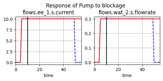
Blockage Fault

We can also look at other faults. The results below are for a blockage of the pipe. In this case we’re only interested in the effect on the water going through, so only those flows are tracked.

endresults2, mdlhist2=propagate.one_fault(mdl, 'export_water', 'block', 
                                          time=10, to_return=['classify', 'graph', 'endfaults'])
summ = mdlhist_full.get_fault_degradation_summary(*mdl.fxns, *mdl.flows)

summ.has_faults

['move_water']

summ.degraded

['move_water', 'ee_1', 'sig_1', 'wat_1', 'wat_2']

fig, ax = endresults2.faulty.tend.graph.draw(figsize=(6,4), withlegend=False)

mdlhist

nominal.i.finished:            array(56)
nominal.i.on:                  array(56)
nominal.m.sub_faults:          array(56)
nominal.time:                  array(56)
nominal.flows.ee_1.s.current:  array(56)
nominal.flows.ee_1.s.voltage:  array(56)
nominal.flows.sig_1.s.power:   array(56)
nominal.flows.wat_1.s.flowrate: array(56)
nominal.flows.wat_1.s.pressure: array(56)
nominal.flows.wat_1.s.area:    array(56)
nominal.flows.wat_1.s.level:   array(56)
nominal.flows.wat_2.s.flowrate: array(56)
nominal.flows.wat_2.s.pressure: array(56)
nominal.flows.wat_2.s.area:    array(56)
nominal.flows.wat_2.s.level:   array(56)
nominal.fxns.import_ee.s.effstate: array(56)
nominal.fxns.import_ee.m.faults.inf_v: array(56)
nominal.fxns.import_ee.m.faults.no_v: array(56)
nominal.fxns.import_ee.m.sub_faults: array(56)
nominal.fxns.import_           array(56)
nominal.fxns.import_           array(56)
nominal.fxns.import_water.m.sub_faults: array(56)
nominal.fxns.import_           array(56)
nominal.fxns.import_           array(56)
nominal.fxns.move_wa           array(56)
nominal.fxns.move_water.s.eff: array(56)
nominal.fxns.move_wa           array(56)
nominal.fxns.move_water.m.faults.short: array(56)
nominal.fxns.move_water.m.sub_faults: array(56)
nominal.fxns.move_wa           array(56)
nominal.fxns.move_wa           array(56)
nominal.fxns.export_           array(56)
nominal.fxns.export_water.m.sub_faults: array(56)
move_water_short_t10.i.finished: array(56)
move_water_short_t10.i.on:     array(56)
move_water_short_t10.m.sub_faults: array(56)
move_water_short_t10.time:     array(56)
move_water_short_t10           array(56)
move_water_short_t10           array(56)
move_water_short_t10           array(56)
move_water_short_t10           array(56)
move_water_short_t10           array(56)
move_water_short_t10           array(56)
move_water_short_t10           array(56)
move_water_short_t10           array(56)
move_water_short_t10           array(56)
move_water_short_t10           array(56)
move_water_short_t10           array(56)
move_water_short_t10           array(56)
move_water_short_t10           array(56)
move_water_short_t10           array(56)
move_water_short_t10           array(56)
move_water_short_t10           array(56)
move_water_short_t10           array(56)
move_water_short_t10           array(56)
move_water_short_t10           array(56)
move_water_short_t10           array(56)
move_water_short_t10           array(56)
move_water_short_t10           array(56)
move_water_short_t10           array(56)
move_water_short_t10           array(56)
move_water_short_t10           array(56)
move_water_short_t10           array(56)
move_water_short_t10           array(56)
move_water_short_t10           array(56)
move_water_short_t10           array(56)

fig, axs = mdlhist2.plot_line('flows.ee_1.s.current', 'flows.wat_2.s.flowrate',
                              title = 'Response of Pump to blockage', time_slice=10, legend_loc=False, title_padding=0.1)

Visualization of resilience metrics

We can also use the processed time history to now make visualizations of the resilience of the system over time.

Here we calculate the percent time the simulation was decraded over the simulation interval:

fxns_and_flows = [*mdl.get_roles_as_dict("fxn", "flow", with_prefix=True)]
deghist = mdlhist_full.get_degraded_hist(*fxns_and_flows)
exp = deghist.get_metrics()

exp

fxns.import_ee:                      0.0
fxns.import_water:                   0.0
fxns.import_signal:                  0.0
fxns.move_water:      0.8214285714285714
fxns.export_water:                   0.0
flows.ee_1:          0.10714285714285714
flows.sig_1:         0.10714285714285714
flows.wat_1:         0.10714285714285714
flows.wat_2:         0.10714285714285714
total:                              1.25
time:                               27.5

These metrics (and others like them) can then be overlayed as a heatmap using set_heatmap.

mg = FunctionArchitectureGraph(mdl)
mg.set_heatmap({mdl.name+"."+k: v for k, v in exp.items()})
mg.draw()

(<Figure size 1200x1000 with 1 Axes>, <Axes: >)

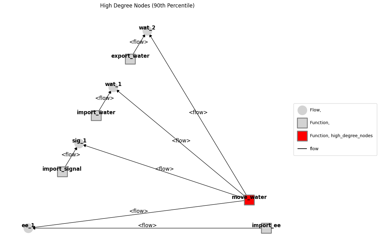
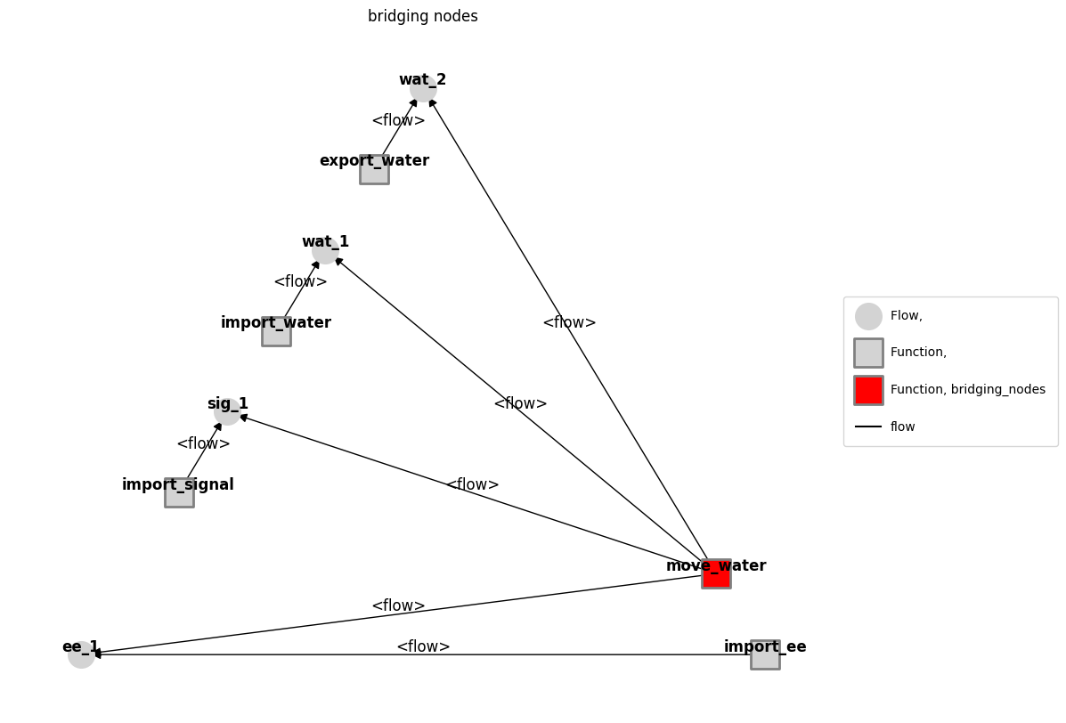
Network metrics can also be overlaid on the graphs:

mg = FunctionArchitectureGraph(mdl)
fig, ax = mg.plot_high_degree_nodes()

mg = FunctionArchitectureGraph(mdl)
fig, ax = mg.plot_bridging_nodes()

Running a List of Faults

Finally, to get the results of all of the single-fault scenarios defined in the model, we can run them all at once using the single_faults() function. Note that this will propagate faults based on the times vector put in the model it will propogate the faults at the begining, end, and at t=15 and t=15. This function only takes in the model mdl and outputs two similar kinds of output–resultsdict (the results in a python dictionary) and resultstab (the results in a nice tabular form).

Note that the rates provide for this table do not use the opportunity vector information, instead using the assumption that the fault scenario has the rate provided over the entire simulation.

See below:

results, mdlhists=propagate.single_faults(mdl, staged=True, track="all")

SCENARIOS COMPLETE: 100%|██████████| 8/8 [00:00<00:00, 15.79it/s]

We can visualize the metrics for each scenario using Result.create_simple_fmea

results.create_simple_fmea()

	rate	cost	expected_cost
nominal	1.000000e+00	0.0	0.00
pump_fxns_import_ee_inf_v_t0p0	0.000000e+00	-26875.0	-0.00
pump_fxns_import_ee_no_v_t0p0	0.000000e+00	-21875.0	-0.00
pump_fxns_import_water_less_wat_t0p0	1.000000e-05	-31875.0	-31875.00
pump_fxns_import_water_no_wat_t0p0	1.000000e-05	-30875.0	-30875.00
pump_fxns_import_signal_no_sig_t0p0	1.500000e-06	-21875.0	-3281.25
pump_fxns_move_water_mech_break_t0p0	6.000000e-07	-26875.0	-1612.50
pump_fxns_move_water_short_t0p0	1.500000e-05	-21875.0	-32812.50
pump_fxns_export_water_block_t0p0	1.500000e-05	-26875.0	-40312.50

We can see corresponding degradations using tabulate.result_summary.fmea()

fullfmea = an.tabulate.result_summary_fmea(results, mdlhists, *mdl.fxns, *mdl.flows)
fullfmea[:10]

	degraded	faulty	rate	cost	expected_cost
nominal	[]	[]	1.0	0.0	0.0
pump_fxns_import_ee_inf_v_t0p0	['import_ee', 'ee_1', 'sig_1', 'wat_1', 'wat_2']	['import_ee']	0.0	-26875.0	-0.0
pump_fxns_import_ee_no_v_t0p0	['import_ee', 'ee_1', 'sig_1', 'wat_1', 'wat_2']	['import_ee']	0.0	-21875.0	-0.0
pump_fxns_import_water_less_wat_t0p0	['import_water', 'ee_1', 'sig_1', 'wat_1', 'wa...	['import_water']	0.00001	-31875.0	-31875.0
pump_fxns_import_water_no_wat_t0p0	['import_water', 'ee_1', 'sig_1', 'wat_1', 'wa...	['import_water']	0.00001	-30875.0	-30875.0
pump_fxns_import_signal_no_sig_t0p0	['import_signal', 'ee_1', 'sig_1', 'wat_1', 'w...	['import_signal']	0.000002	-21875.0	-3281.25
pump_fxns_move_water_mech_break_t0p0	['move_water', 'ee_1', 'sig_1', 'wat_1', 'wat_2']	['move_water']	0.000001	-26875.0	-1612.5
pump_fxns_move_water_short_t0p0	['move_water', 'ee_1', 'sig_1', 'wat_1', 'wat_2']	['move_water']	0.000015	-21875.0	-32812.5
pump_fxns_export_water_block_t0p0	['export_water', 'ee_1', 'sig_1', 'wat_1', 'wa...	['export_water']	0.000015	-26875.0	-40312.5

Running a Fault Sampling Approach

Note that only gives accurate results for costs and fault responses–in order to get an accurate idea of expected cost, we instead run a FaultSample or SampleApproach, which develops an underlying probability model for faults. See below.

from fmdtools.sim.sample import FaultDomain, FaultSample

fd = FaultDomain(mdl)
fd.add_all()
fd

FaultDomain with faults:
 -('pump.fxns.import_ee', 'inf_v')
 -('pump.fxns.import_ee', 'no_v')
 -('pump.fxns.import_water', 'less_wat')
 -('pump.fxns.import_water', 'no_wat')
 -('pump.fxns.import_signal', 'no_sig')
 -('pump.fxns.move_water', 'mech_break')
 -('pump.fxns.move_water', 'short')
 -('pump.fxns.export_water', 'block')

from fmdtools.analyze.phases import PhaseMap
fs = FaultSample(fd, phasemap=PhaseMap(mdl.sp.phases))
fs.add_fault_phases()
fs

FaultSample of scenarios: 
 - pump_fxns_import_ee_inf_v_t2p0
 - pump_fxns_import_ee_no_v_t2p0
 - pump_fxns_import_water_less_wat_t2p0
 - pump_fxns_import_water_no_wat_t2p0
 - pump_fxns_import_signal_no_sig_t2p0
 - pump_fxns_move_water_mech_break_t2p0
 - pump_fxns_move_water_short_t2p0
 - pump_fxns_export_water_block_t2p0
 - pump_fxns_import_ee_inf_v_t27p0
 - pump_fxns_import_ee_no_v_t27p0
 - ... (24 total)

results, mdlhists=propagate.fault_sample(mdl, fs, staged=True, track="all")
simplefmea = results.create_simple_fmea() #note the costs are the same, but the rates and expected costs are not
simplefmea[:5]

SCENARIOS COMPLETE: 100%|██████████| 24/24 [00:00<00:00, 31.01it/s]

	rate	cost	expected_cost
nominal	1.00000	0.0	0.0
pump_fxns_import_ee_inf_v_t2p0	0.00000	15125.0	0.0
pump_fxns_import_ee_no_v_t2p0	0.00000	20125.0	0.0
pump_fxns_import_water_less_wat_t2p0	0.00001	10125.0	10125.0
pump_fxns_import_water_no_wat_t2p0	0.00001	11125.0	11125.0

We can now summarize the risks of faults over the operational phases and overall using the FMEA class:

phasefmea = an.tabulate.FMEA(results, fs, group_by=('obj', 'fault', 'phase'))
phasefmea.as_table()

			average_scenario_rate	sum_cost	expected_cost
pump.fxns.move_water	short	start	1.500000e-05	20125.0	0.301875
pump.fxns.export_water	block	start	1.500000e-05	15125.0	0.226875
pump.fxns.import_water	no_wat	start	1.000000e-05	11125.0	0.111250
	less_wat	start	1.000000e-05	10125.0	0.101250
pump.fxns.move_water	short	end	1.000000e-05	10000.0	0.100000
		on	1.000000e-05	8650.0	0.086500
pump.fxns.import_ee	no_v	on	8.000000e-06	8650.0	0.069200
pump.fxns.export_water	block	end	1.000000e-05	5000.0	0.050000
		on	1.000000e-05	3650.0	0.036500
pump.fxns.import_signal	no_sig	start	1.500000e-06	20125.0	0.030188
pump.fxns.move_water	mech_break	on	7.200000e-06	3650.0	0.026280
pump.fxns.import_signal	no_sig	end	1.000000e-06	10000.0	0.010000
pump.fxns.import_water	no_wat	end	1.000000e-05	1000.0	0.010000
pump.fxns.move_water	mech_break	start	6.000000e-07	15125.0	0.009075
pump.fxns.import_signal	no_sig	on	1.000000e-06	8650.0	0.008650
pump.fxns.import_ee	inf_v	on	2.000000e-06	3650.0	0.007300
pump.fxns.move_water	mech_break	end	6.000000e-07	5000.0	0.003000
pump.fxns.import_ee	no_v	end	0.000000e+00	10000.0	0.000000
	inf_v	end	0.000000e+00	5000.0	0.000000
	no_v	start	0.000000e+00	20125.0	0.000000
pump.fxns.import_water	less_wat	end	1.000000e-05	0.0	0.000000
pump.fxns.import_ee	inf_v	start	0.000000e+00	15125.0	0.000000
pump.fxns.import_water	no_wat	on	1.000000e-05	-350.0	-0.003500
	less_wat	on	1.000000e-05	-1350.0	-0.013500

summfmea = an.tabulate.FMEA(results, fs)
summfmea.as_table()

		average_scenario_rate	sum_cost	expected_cost
pump.fxns.move_water	short	1.166667e-05	38775.0	0.488375
pump.fxns.export_water	block	1.166667e-05	23775.0	0.313375
pump.fxns.import_water	no_wat	1.000000e-05	11775.0	0.117750
	less_wat	1.000000e-05	8775.0	0.087750
pump.fxns.import_ee	no_v	2.666667e-06	38775.0	0.069200
pump.fxns.import_signal	no_sig	1.166667e-06	38775.0	0.048838
pump.fxns.move_water	mech_break	2.800000e-06	23775.0	0.038355
pump.fxns.import_ee	inf_v	6.666667e-07	23775.0	0.007300

History visualization

We can further overlay expected resilience metrics on the model over fault scenarios using various methods provided with History and Result.

Below we get the expected values of the history values:

hist_expected = mdlhists.get_expected(app=fs, with_nominal=True)

Next we get the expected degradations:

deg=hist_expected.get_degraded_hist(*fxns_and_flows, nomhist=mdlhists.nominal)

deg

fxns.import_ee:                array(56)
fxns.move_water:               array(56)
flows.ee_1:                    array(56)
flows.sig_1:                   array(56)
flows.wat_1:                   array(56)
flows.wat_2:                   array(56)
total:                         array(56)
time:                          array(56)

import numpy as np
heatmap = deg.get_metrics(metric=np.mean)
heatmap

fxns.import_ee:       0.9642857142857143
fxns.move_water:      0.9642857142857143
flows.ee_1:                          1.0
flows.sig_1:          0.9107142857142857
flows.wat_1:          0.9107142857142857
flows.wat_2:          0.9107142857142857
total:                 5.660714285714286
time:                               27.5

These metrics can in turn be overlayed on the graph using set_heatmap.

from fmdtools.define.architecture.function import FunctionArchitectureGraph
mg = FunctionArchitectureGraph(mdl)
hm = {}
for k, v in heatmap.items():
    if k in mdl.flows:
        k2 = mdl.name+'.flows.'+k
        hm[k2] = v
    elif k in mdl.fxns:
        k2 = mdl.name+'.fxns.'+k
        hm[k2] = v
mg.set_heatmap(hm)
mg.draw()

(<Figure size 1200x1000 with 1 Axes>, <Axes: >)

Save/Load

In detailed simulations, running a lot of computational simulations can take a considerable amount of time. As a result, it becomes impractical to run a new simulation every time one wishes to analyse its data. Results from fmdtools simulations (results or histories) can be saved as npz, csv, or json files in this instance using either:

• Result.save or History.save or

• passing a save_args dictionary to the respective propagate functions (e.g., {‘classify’:{‘filename’:’file.pkl’,’overwrite’:True})

and then loaded using:

• Result.load or History.load

mdlhists

nominal.i.finished:            array(56)
nominal.i.on:                  array(56)
nominal.m.sub_faults:          array(56)
nominal.time:                  array(56)
nominal.flows.ee_1.s.current:  array(56)
nominal.flows.ee_1.s.voltage:  array(56)
nominal.flows.sig_1.s.power:   array(56)
nominal.flows.wat_1.s.flowrate: array(56)
nominal.flows.wat_1.s.pressure: array(56)
nominal.flows.wat_1.s.area:    array(56)
nominal.flows.wat_1.s.level:   array(56)
nominal.flows.wat_2.s.flowrate: array(56)
nominal.flows.wat_2.s.pressure: array(56)
nominal.flows.wat_2.s.area:    array(56)
nominal.flows.wat_2.s.level:   array(56)
nominal.fxns.import_ee.s.effstate: array(56)
nominal.fxns.import_ee.m.faults.inf_v: array(56)
nominal.fxns.import_ee.m.faults.no_v: array(56)
nominal.fxns.import_ee.m.sub_faults: array(56)
nominal.fxns.import_           array(56)
nominal.fxns.import_           array(56)
nominal.fxns.import_water.m.sub_faults: array(56)
nominal.fxns.import_           array(56)
nominal.fxns.import_           array(56)
nominal.fxns.move_wa           array(56)
nominal.fxns.move_water.s.eff: array(56)
nominal.fxns.move_wa           array(56)
nominal.fxns.move_water.m.faults.short: array(56)
nominal.fxns.move_water.m.sub_faults: array(56)
nominal.fxns.move_wa           array(56)
nominal.fxns.move_wa           array(56)
nominal.fxns.export_           array(56)
nominal.fxns.export_water.m.sub_faults: array(56)
pump_fxns_import_ee_           array(56)
pump_fxns_import_ee_inf_v_t2p0.i.on: array(56)
pump_fxns_import_ee_           array(56)
pump_fxns_import_ee_inf_v_t2p0.time: array(56)
pump_fxns_import_ee_           array(56)
pump_fxns_import_ee_           array(56)
pump_fxns_import_ee_           array(56)
pump_fxns_import_ee_           array(56)
pump_fxns_import_ee_           array(56)
pump_fxns_import_ee_           array(56)
pump_fxns_import_ee_           array(56)
pump_fxns_import_ee_           array(56)
pump_fxns_import_ee_           array(56)
pump_fxns_import_ee_           array(56)
pump_fxns_import_ee_           array(56)
pump_fxns_import_ee_           array(56)
pump_fxns_import_ee_           array(56)
pump_fxns_import_ee_           array(56)
pump_fxns_import_ee_           array(56)
pump_fxns_import_ee_           array(56)
pump_fxns_import_ee_           array(56)
pump_fxns_import_ee_           array(56)
pump_fxns_import_ee_           array(56)
pump_fxns_import_ee_           array(56)
pump_fxns_import_ee_           array(56)
pump_fxns_import_ee_           array(56)
pump_fxns_import_ee_           array(56)
pump_fxns_import_ee_           array(56)
pump_fxns_import_ee_           array(56)
pump_fxns_import_ee_           array(56)
pump_fxns_import_ee_           array(56)
pump_fxns_import_ee_           array(56)
pump_fxns_import_ee_           array(56)
pump_fxns_import_ee_           array(56)
pump_fxns_import_ee_no_v_t2p0.i.on: array(56)
pump_fxns_import_ee_           array(56)
pump_fxns_import_ee_no_v_t2p0.time: array(56)
pump_fxns_import_ee_           array(56)
pump_fxns_import_ee_           array(56)
pump_fxns_import_ee_           array(56)
pump_fxns_import_ee_           array(56)
pump_fxns_import_ee_           array(56)
pump_fxns_import_ee_           array(56)
pump_fxns_import_ee_           array(56)
pump_fxns_import_ee_           array(56)
pump_fxns_import_ee_           array(56)
pump_fxns_import_ee_           array(56)
pump_fxns_import_ee_           array(56)
pump_fxns_import_ee_           array(56)
pump_fxns_import_ee_           array(56)
pump_fxns_import_ee_           array(56)
pump_fxns_import_ee_           array(56)
pump_fxns_import_ee_           array(56)
pump_fxns_import_ee_           array(56)
pump_fxns_import_ee_           array(56)
pump_fxns_import_ee_           array(56)
pump_fxns_import_ee_           array(56)
pump_fxns_import_ee_           array(56)
pump_fxns_import_ee_           array(56)
pump_fxns_import_ee_           array(56)
pump_fxns_import_ee_           array(56)
pump_fxns_import_ee_           array(56)
pump_fxns_import_ee_           array(56)
pump_fxns_import_ee_           array(56)
pump_fxns_import_ee_           array(56)
pump_fxns_import_ee_           array(56)
 ...825 lines

This saves a history to a file:

mdlhists.save("outputs_demo_fault_analysis/example_mdlhist.npz", overwrite=True)

File already exists: outputs_demo_fault_analysis/example_mdlhist.npz, writing anyway...

And this loads this history:

mdlhists_saved  = an.history.History.load("outputs_demo_fault_analysis/example_mdlhist.npz")

mdlhists_saved 

nominal.i.finished:            array(56)
nominal.i.on:                  array(56)
nominal.m.sub_faults:          array(56)
nominal.time:                  array(56)
nominal.flows.ee_1.s.current:  array(56)
nominal.flows.ee_1.s.voltage:  array(56)
nominal.flows.sig_1.s.power:   array(56)
nominal.flows.wat_1.s.flowrate: array(56)
nominal.flows.wat_1.s.pressure: array(56)
nominal.flows.wat_1.s.area:    array(56)
nominal.flows.wat_1.s.level:   array(56)
nominal.flows.wat_2.s.flowrate: array(56)
nominal.flows.wat_2.s.pressure: array(56)
nominal.flows.wat_2.s.area:    array(56)
nominal.flows.wat_2.s.level:   array(56)
nominal.fxns.import_ee.s.effstate: array(56)
nominal.fxns.import_ee.m.faults.inf_v: array(56)
nominal.fxns.import_ee.m.faults.no_v: array(56)
nominal.fxns.import_ee.m.sub_faults: array(56)
nominal.fxns.import_           array(56)
nominal.fxns.import_           array(56)
nominal.fxns.import_water.m.sub_faults: array(56)
nominal.fxns.import_           array(56)
nominal.fxns.import_           array(56)
nominal.fxns.move_wa           array(56)
nominal.fxns.move_water.s.eff: array(56)
nominal.fxns.move_wa           array(56)
nominal.fxns.move_water.m.faults.short: array(56)
nominal.fxns.move_water.m.sub_faults: array(56)
nominal.fxns.move_wa           array(56)
nominal.fxns.move_wa           array(56)
nominal.fxns.export_           array(56)
nominal.fxns.export_water.m.sub_faults: array(56)
pump_fxns_import_ee_           array(56)
pump_fxns_import_ee_inf_v_t2p0.i.on: array(56)
pump_fxns_import_ee_           array(56)
pump_fxns_import_ee_inf_v_t2p0.time: array(56)
pump_fxns_import_ee_           array(56)
pump_fxns_import_ee_           array(56)
pump_fxns_import_ee_           array(56)
pump_fxns_import_ee_           array(56)
pump_fxns_import_ee_           array(56)
pump_fxns_import_ee_           array(56)
pump_fxns_import_ee_           array(56)
pump_fxns_import_ee_           array(56)
pump_fxns_import_ee_           array(56)
pump_fxns_import_ee_           array(56)
pump_fxns_import_ee_           array(56)
pump_fxns_import_ee_           array(56)
pump_fxns_import_ee_           array(56)
pump_fxns_import_ee_           array(56)
pump_fxns_import_ee_           array(56)
pump_fxns_import_ee_           array(56)
pump_fxns_import_ee_           array(56)
pump_fxns_import_ee_           array(56)
pump_fxns_import_ee_           array(56)
pump_fxns_import_ee_           array(56)
pump_fxns_import_ee_           array(56)
pump_fxns_import_ee_           array(56)
pump_fxns_import_ee_           array(56)
pump_fxns_import_ee_           array(56)
pump_fxns_import_ee_           array(56)
pump_fxns_import_ee_           array(56)
pump_fxns_import_ee_           array(56)
pump_fxns_import_ee_           array(56)
pump_fxns_import_ee_           array(56)
pump_fxns_import_ee_           array(56)
pump_fxns_import_ee_no_v_t2p0.i.on: array(56)
pump_fxns_import_ee_           array(56)
pump_fxns_import_ee_no_v_t2p0.time: array(56)
pump_fxns_import_ee_           array(56)
pump_fxns_import_ee_           array(56)
pump_fxns_import_ee_           array(56)
pump_fxns_import_ee_           array(56)
pump_fxns_import_ee_           array(56)
pump_fxns_import_ee_           array(56)
pump_fxns_import_ee_           array(56)
pump_fxns_import_ee_           array(56)
pump_fxns_import_ee_           array(56)
pump_fxns_import_ee_           array(56)
pump_fxns_import_ee_           array(56)
pump_fxns_import_ee_           array(56)
pump_fxns_import_ee_           array(56)
pump_fxns_import_ee_           array(56)
pump_fxns_import_ee_           array(56)
pump_fxns_import_ee_           array(56)
pump_fxns_import_ee_           array(56)
pump_fxns_import_ee_           array(56)
pump_fxns_import_ee_           array(56)
pump_fxns_import_ee_           array(56)
pump_fxns_import_ee_           array(56)
pump_fxns_import_ee_           array(56)
pump_fxns_import_ee_           array(56)
pump_fxns_import_ee_           array(56)
pump_fxns_import_ee_           array(56)
pump_fxns_import_ee_           array(56)
pump_fxns_import_ee_           array(56)
pump_fxns_import_ee_           array(56)
pump_fxns_import_ee_           array(56)
 ...825 lines

Note that there are different trade-offs to using different file formats:

• npz is the serialization format provided in numpy, which is fast but not human readable

• csv outputs as comma separated values, which are slower and less robust (in terms of data types), but are human-readable and can be opened in a spreadsheet software like excel.

• json is similar to csv, but is less human readable.