EPS Example Notebook

This notebook shows how fmdtools can be used for static propagation models. Static propagation models are meant to represent events occurring within a time-step (as opposed to over several timesteps). The electric power system used as an examples replicates a previous power system case study implemented in IBFM, and also showcases some basic fault propagation and visualization.

Copyright © 2024, United States Government, as represented by the Administrator of the National Aeronautics and Space Administration. All rights reserved.

The “"Fault Model Design tools - fmdtools version 2"” software is licensed under the Apache License, Version 2.0 (the "License"); you may not use this file except in compliance with the License. You may obtain a copy of the License at http://www.apache.org/licenses/LICENSE-2.0. 

Unless required by applicable law or agreed to in writing, software distributed under the License is distributed on an "AS IS" BASIS, WITHOUT WARRANTIES OR CONDITIONS OF ANY KIND, either express or implied. See the License for the specific language governing permissions and limitations under the License.

from fmdtools_examples.electric_power_system.model_main import EPS
import fmdtools.sim.propagate as propagate

This script provides some example I/O for using static models, using the EPS system implemented in eps.py as an example.

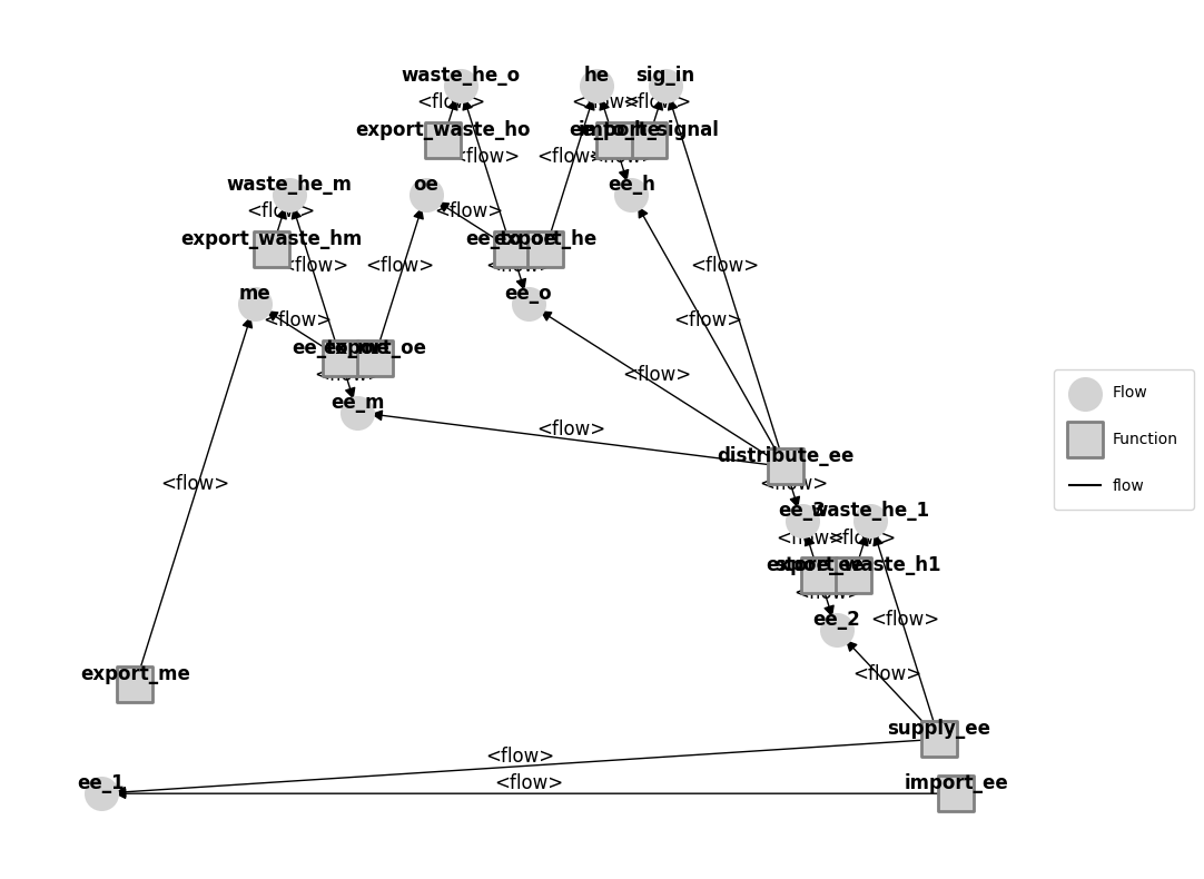
A graphical representaiton of this system is shown below:

mdl= EPS()
mg = mdl.as_modelgraph()
fig, ax = mg.draw()

As with dynamic models, in static models we use fp.run_one_fault to see the effects of single faults. All setup is performed in the Model class definition

result, mdlhist = propagate.one_fault(mdl, 'ee_to_me', 'toohigh_torque', to_return=["graph"])

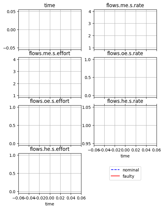
In this case, however, the output in mdlhists will be a single-dimensional dictionary (not something we can plot very well)

fig, ax = mdlhist.plot_line(*mdlhist.nominal.keys())

C:\Users\dhulse\Documents\GitHub\fmdtools\src\fmdtools\analyze\common.py:547: UserWarning: Attempting to set identical low and high xlims makes transformation singular; automatically expanding.
  ax.set_xlim(*xlim)

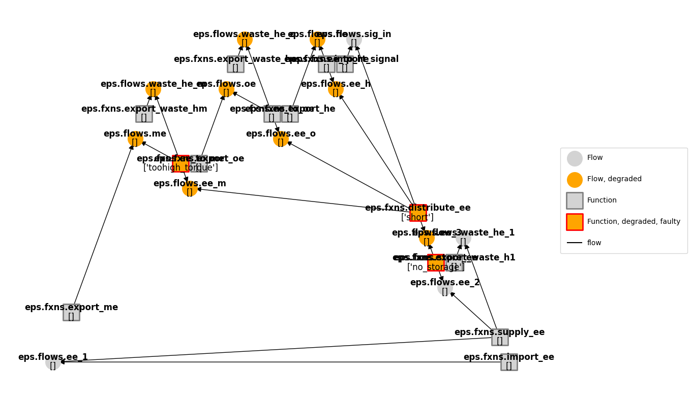
As a result, it’s better to look at the results graph for a visualization of what went wrong. In this case resgraph better represents the fault propagation of the system than in a dynamic model, since there is only one time-step to represent (rather than a set)

graph = result.get_faulty().tend.graph
graph.set_edge_labels(title='')
fig, ax = graph.draw(figsize=(14,10))

We can run the set of single-fault scenarios on this model using fmdtools.sim.propagate.single_faults. For single-fault scenarios, one does not need to use a SampleApproach, since all faults are injected at a single time-step.

mdl= EPS(track='all')
results, mdlhists = propagate.single_faults(mdl, staged=True)

SCENARIOS COMPLETE: 100%|██████████| 35/35 [00:00<00:00, 75.36it/s]

Using analyze.tabulate.result_summary_fmea, one can see the degradation effects of this fault on the flows:

from fmdtools.analyze.tabulate import result_summary_fmea

tab = result_summary_fmea(results, mdlhists, *mdl.fxns, *mdl.flows)
tab.sort_values("expected_cost")

	degraded	faulty	rate	cost	expected_cost
nominal	[]	[]	1.0	0.0	0.0
eps_fxns_ee_to_he_open_circuit_t0p0	['ee_to_he', 'ee_h', 'he']	['ee_to_he']	0.0	550.0	2.409
eps_fxns_supply_ee_open_circuit_t0p0	['supply_ee', 'ee_2', 'ee_3', 'ee_m', 'ee_o', ...	['supply_ee']	0.0	1450.0	3.1755
eps_fxns_ee_to_he_high_heat_t0p0	['supply_ee', 'store_ee', 'ee_to_he', 'ee_2', ...	['supply_ee', 'store_ee', 'ee_to_he']	0.0	2500.0	10.95
eps_fxns_ee_to_oe_optical_resist_t0p0	['ee_to_oe', 'ee_o', 'oe', 'he', 'waste_he_o']	['ee_to_oe']	0.0	520.0	11.388
eps_fxns_supply_ee_short_t0p0	['supply_ee', 'store_ee', 'distribute_ee', 'ee...	['supply_ee', 'store_ee', 'distribute_ee']	0.0	5150.0	22.557
eps_fxns_ee_to_he_low_heat_t0p0	['ee_to_he', 'he']	['ee_to_he']	0.000002	550.0	48.18
eps_fxns_ee_to_oe_burnt_out_t0p0	['ee_to_oe', 'ee_o', 'oe', 'he', 'waste_he_o']	['ee_to_oe']	0.000002	550.0	48.18
eps_fxns_import_signal_no_signal_t0p0	['import_signal', 'ee_2', 'ee_3', 'ee_m', 'ee_...	['import_signal']	0.000001	2000.0	87.6
eps_fxns_ee_to_he_toohigh_heat_t0p0	['store_ee', 'distribute_ee', 'ee_to_he', 'ee_...	['store_ee', 'distribute_ee', 'ee_to_he']	0.0	5100.0	111.69
eps_fxns_supply_ee_adverse_resist_t0p0	['supply_ee', 'ee_2', 'ee_3', 'ee_m', 'ee_o', ...	['supply_ee']	0.000002	1650.0	144.54
eps_fxns_export_waste_ho_ineffective_sink_t0p0	['export_waste_ho', 'he', 'waste_he_o']	['export_waste_ho']	0.000005	1000.0	219.0
eps_fxns_export_waste_ho_hot_sink_t0p0	['export_waste_ho', 'he', 'waste_he_o']	['export_waste_ho']	0.00001	500.0	219.0
eps_fxns_export_waste_h1_ineffective_sink_t0p0	['export_waste_h1', 'he', 'waste_he_1']	['export_waste_h1']	0.000005	1000.0	219.0
eps_fxns_export_waste_h1_hot_sink_t0p0	['export_waste_h1', 'he', 'waste_he_1']	['export_waste_h1']	0.00001	500.0	219.0
eps_fxns_export_waste_hm_hot_sink_t0p0	['export_waste_hm', 'he', 'waste_he_m']	['export_waste_hm']	0.00001	500.0	219.0
eps_fxns_export_waste_hm_ineffective_sink_t0p0	['export_waste_hm', 'he', 'waste_he_m']	['export_waste_hm']	0.000005	1000.0	219.0
eps_fxns_export_he_hot_sink_t0p0	['export_he', 'he']	['export_he']	0.00001	600.0	262.8
eps_fxns_import_ee_low_v_t0p0	['import_ee', 'ee_1', 'ee_2', 'ee_3', 'ee_m', ...	['import_ee']	0.00001	700.0	306.6
eps_fxns_export_he_ineffective_sink_t0p0	['export_he', 'he']	['export_he']	0.000005	1500.0	328.5
eps_fxns_supply_ee_major_overload_t0p0	['supply_ee', 'store_ee', 'ee_2', 'he', 'waste...	['supply_ee', 'store_ee']	0.000003	2600.0	341.64
eps_fxns_store_ee_low_storage_t0p0	['store_ee']	['store_ee']	0.000005	2000.0	438.0
eps_fxns_import_ee_high_v_t0p0	['import_ee', 'supply_ee', 'store_ee', 'ee_1',...	['import_ee', 'supply_ee', 'store_ee']	0.000005	2300.0	503.7
eps_fxns_import_ee_no_v_t0p0	['import_ee', 'ee_1', 'ee_2', 'ee_3', 'ee_m', ...	['import_ee']	0.00001	1550.0	678.9
eps_fxns_store_ee_no_storage_t0p0	['store_ee', 'ee_3', 'ee_m', 'ee_o', 'ee_h', '...	['store_ee']	0.000005	3250.0	711.75
eps_fxns_import_signal_partial_signal_t0p0	['import_signal', 'ee_2', 'ee_3', 'ee_m', 'ee_...	['import_signal']	0.00001	2000.0	876.0
eps_fxns_distribute_ee_adverse_resist_t0p0	['distribute_ee', 'ee_2', 'ee_3', 'ee_m', 'ee_...	['distribute_ee']	0.00001	2750.0	1204.5
eps_fxns_ee_to_me_open_circuit_t0p0	['ee_to_me', 'ee_m', 'me', 'he', 'waste_he_m']	['ee_to_me']	0.00005	650.0	1423.5
eps_fxns_distribute_ee_poor_alloc_t0p0	['distribute_ee', 'ee_2', 'ee_3', 'ee_m', 'ee_...	['distribute_ee']	0.00002	1750.0	1533.0
eps_fxns_ee_to_me_high_torque_t0p0	['ee_to_me', 'ee_m', 'me', 'he', 'waste_he_m']	['ee_to_me']	0.0001	450.0	1971.0
eps_fxns_supply_ee_minor_overload_t0p0	['supply_ee', 'store_ee', 'distribute_ee', 'ee...	['supply_ee', 'store_ee', 'distribute_ee']	0.00001	5150.0	2255.7
eps_fxns_distribute_ee_open_circuit_t0p0	['distribute_ee', 'ee_2', 'ee_3', 'ee_m', 'ee_...	['distribute_ee']	0.00003	2750.0	3613.5
eps_fxns_distribute_ee_short_t0p0	['store_ee', 'distribute_ee', 'ee_3', 'ee_m', ...	['store_ee', 'distribute_ee']	0.00002	4750.0	4161.0
eps_fxns_ee_to_me_short_t0p0	['store_ee', 'distribute_ee', 'ee_to_me', 'ee_...	['store_ee', 'distribute_ee', 'ee_to_me']	0.00005	4950.0	10840.5
eps_fxns_ee_to_me_toohigh_torque_t0p0	['store_ee', 'distribute_ee', 'ee_to_me', 'ee_...	['store_ee', 'distribute_ee', 'ee_to_me']	0.00005	5050.0	11059.5
eps_fxns_ee_to_me_low_torque_t0p0	['store_ee', 'distribute_ee', 'ee_to_me', 'ee_...	['store_ee', 'distribute_ee', 'ee_to_me']	0.0001	4950.0	21681.0