Demo: Rover Response Optimization
This notebook shows how variables in an fmdtools model can be optimized for resilience.
Copyright © 2024, United States Government, as represented by the Administrator of the National Aeronautics and Space Administration. All rights reserved.

The “"Fault Model Design tools - fmdtools version 2"” software is licensed under the Apache License, Version 2.0 (the "License"); you may not use this file except in compliance with the License. You may obtain a copy of the License at http://www.apache.org/licenses/LICENSE-2.0.

Unless required by applicable law or agreed to in writing, software distributed under the License is distributed on an "AS IS" BASIS, WITHOUT WARRANTIES OR CONDITIONS OF ANY KIND, either express or implied. See the License for the specific language governing permissions and limitations under the License.
from fmdtools.sim.sample import SampleApproach, FaultSample, FaultDomain, ParameterDomain
import fmdtools.analyze as an
import fmdtools.sim.propagate as prop
from fmdtools.sim.search import ParameterSimProblem
import matplotlib.pyplot as plt
import multiprocessing as mp
import time
Model is in defined model_main.py
from fmdtools_examples.navigating_rover.model_main import Rover, RoverParam
Optimization
Here we define the optimization problem for the rover.
We use a parallel pool, staged execution, and minimal tracking options to lower computational cost as much as possible.
mdl = Rover(sp={'end_condition': ''}, track={'flows':{"ground":"all", "pos": "all"}})
#rover_prob = search.ProblemInterface("rover_problem", mdl, pool=mp.Pool(5), staged=True, track=track)
mdl.h
time:                         array(151)
flows.ground.r.probdens:      array(151)
flows.ground.s.in_bound:      array(151)
flows.ground.sp.phases:       array(151)
flows.ground.sp.start_time:   array(151)
flows.ground.sp.end_time:     array(151)
flows.ground.sp.track_times:  array(151)
flows.ground.sp.dt:           array(151)
flows.ground.sp.units:        array(151)
flows.ground.sp.end_condition: array(151)
flows.ground.sp.use_local:    array(151)
flows.ground.sp.with_loadings: array(151)
flows.ground.sp.run_stochastic: array(151)
flows.ground.sp.track_pdf:    array(151)
flows.ground.c.r.probdens:    array(151)
flows.ground.ga.points.start.s.on: array(151)
flows.ground.ga.points.start.s.near: array(151)
flows.ground.ga.points.end.s.on: array(151)
flows.ground.ga.points.end.s.near: array(151)
flows.pos.s.x:                array(151)
flows.pos.s.y:                array(151)
flows.pos.s.vel:              array(151)
flows.pos.s.ux:               array(151)
flows.pos.s.uy:               array(151)
mdl.p
RoverParam(ground=GroundParam(linetype='sine', amp=1.0, period=6.283185307179586, radius=20.0, x_start=10.0, y_end=10.0, x_min=0.0, x_max=30.0, x_res=0.1, path_buffer_on=0.2, path_buffer_poor=0.3, path_buffer_near=0.4, dest_buffer_on=1.0, dest_buffer_near=2.0), correction=ResCorrection(ub_f=10.0, lb_f=-1.0, ub_t=10.0, lb_t=0.0, ub_d=2.0, lb_d=-2.0, cor_d=0.0, cor_t=0.0, cor_f=0.0), degradation=DegParam(friction=0.0, drift=0.0), drive_modes={'mode_options': 'set'})
Here we will be optimizing over faults in the drive system at 3 points during the drive simulation interval:
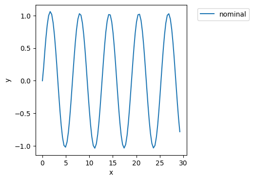
endresults, mdlhist = prop.nominal(Rover())
phasemap = an.phases.from_hist(mdlhist)
fault_domain = FaultDomain(mdl)
fault_domain.add_all_fxnclass_modes('Drive')
fault_sample = FaultSample(fault_domain, phasemap['plan_path'])
fault_sample.add_fault_phases('drive',  args=(3,))
fig, ax = mdlhist.plot_trajectories("flows.pos.s.x", "flows.pos.s.y")
The variables are the correction factors int the fault management:
pd = ParameterDomain(RoverParam)
pd.add_variables("correction.cor_f", "correction.cor_d", "correction.cor_t", lims={"correction.cor_f":(0, 1),
                                                                                         "correction.cor_d":(-1, 1),
                                                                                         "correction.cor_t":(-1, 1)})
pd
ParameterDomain with:
 - variables: {'correction.cor_f': (0, 1), 'correction.cor_d': (-1, 1), 'correction.cor_t': (-1, 1)}
 - constants: {}
 - parameter_initializer: RoverParam
Now we setup the optimization problem using ParameterSimProblem
We can define multiple objectives, below we will use the end distance and total_deviation from classify.
class RoverProb(ParameterSimProblem):
    def init_problem(self, **kwargs):
        self.add_parameterdomain(pd)
        self.add_sim(mdl, "fault_sample", fault_sample, **kwargs)
        self.add_result_objective('f1', 'classify.end_dist')
        self.add_result_objective('f2', 'classify.tot_deviation')
rover_prob = RoverProb()
rover_prob
RoverProb with:
VARIABLES
 -correction.cor_f                                              nan
 -correction.cor_d                                              nan
 -correction.cor_t                                              nan
OBJECTIVES
 -f1                                                            nan
 -f2                                                            nan
Here we do some basic timing:
rover_prob.f1(0.5,0.5,0.5)
a=time.time()
rover_prob.f1(0.6,0.5,0.5)
t=time.time()-a
t
4.043263912200928
rover_prob
RoverProb with:
VARIABLES
 -correction.cor_f                                           0.6000
 -correction.cor_d                                           0.5000
 -correction.cor_t                                           0.5000
OBJECTIVES
 -f1                                                       129.8820
 -f2                                                         2.5205
Alternatively, we can use:
rover_prob.time_execution(0.7,0.5,0.5)
4.076462268829346
fig, ax = rover_prob.hist.plot_trajectories("flows.pos.s.x", "flows.pos.s.y")
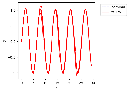
rover_prob
RoverProb with:
VARIABLES
 -correction.cor_f                                           0.7000
 -correction.cor_d                                           0.5000
 -correction.cor_t                                           0.5000
OBJECTIVES
 -f1                                                       132.2823
 -f2                                                         2.5270
Rover Optimization:
from pymoo.optimize import minimize
from pymoo.algorithms.soo.nonconvex.pattern import PatternSearch
from pymoo.problems.functional import FunctionalProblem
import numpy as np
Covert optimization problem into a pymoo problem
from multiprocessing import Pool
rover_prob = RoverProb(pool=Pool(4), auto_close_pool=False)

n_var = len(rover_prob.variables)
x_low = np.array([])
x_up = np.array([])
for bound in rover_prob.parameterdomain.variables.values():
    x_low = np.append(x_low, bound[0])
    x_up = np.append(x_up, bound[1])

obj = [lambda x: rover_prob.f1(*x)]
pymoo_prob = FunctionalProblem(n_var, obj, xl = x_low, xu= x_up)
arg={}
pymoo_prob._evaluate([0.7,0.5,0.5],arg)
arg
{'F': array([132.28226465]),
 'G': array([], dtype=float64),
 'H': array([], dtype=float64)}
Run optimizaion algorithm..
algorithm=PatternSearch(x0=np.array([0.7,0.5,0.5]))
from pymoo.termination import get_termination
# early termination
termination = get_termination("n_eval", 13)
res = minimize(pymoo_prob, algorithm, termination=termination, verbose=True)
=================================================
n_gen  |  n_eval  |     f_avg     |     f_min
=================================================
     1 |        1 |  1.322823E+02 |  1.322823E+02
     2 |        7 |  1.307473E+02 |  1.292124E+02
     3 |       13 |  1.268410E+02 |  1.244696E+02
res.X
array([0.325, 0.5 , 0.5 ])
opt_x = [ 0.16970361, -0.78522209, 0.10777078]
Results visualization
Here we look at the optimized results and compare with the starting results:
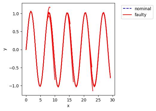
rover_prob.f1(0.16970361, -0.78522209, 0.10777078)
np.float64(122.37205579225862)
fig, ax = rover_prob.hist.plot_trajectories("flows.pos.s.x", "flows.pos.s.y")
rover_prob
RoverProb with:
VARIABLES
 -correction.cor_f                                           0.1697
 -correction.cor_d                                          -0.7852
 -correction.cor_t                                           0.1078
OBJECTIVES
 -f1                                                       122.3721
 -f2                                                         2.5435
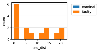
fig, ax = rover_prob.res.plot_metric_dist('end_dist')
starting solution:
rover_prob.f1(0.7,0.5,0.5)
np.float64(132.28226465048797)
fig, ax = rover_prob.hist.plot_trajectories("flows.pos.s.x", "flows.pos.s.y")
rover_prob
RoverProb with:
VARIABLES
 -correction.cor_f                                           0.7000
 -correction.cor_d                                           0.5000
 -correction.cor_t                                           0.5000
OBJECTIVES
 -f1                                                       132.2823
 -f2                                                         2.5270
fig, ax = rover_prob.res.plot_metric_dist('end_dist')
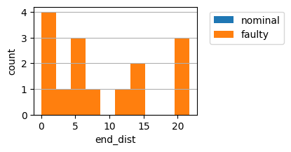
As shown, while the optimized correction factors don’t mitigate all scenarios, they do increase the number of scenarios that are mitigated.
rover_prob.close_pool()