Tutorial: fmdtools basics
::: {.content-hidden}
Copyright © 2024, United States Government, as represented by the Administrator of the National Aeronautics and Space Administration. All rights reserved.

The “"Fault Model Design tools - fmdtools version 2"” software is licensed under the Apache License, Version 2.0 (the "License"); you may not use this file except in compliance with the License. You may obtain a copy of the License at http://www.apache.org/licenses/LICENSE-2.0.

Unless required by applicable law or agreed to in writing, software distributed under the License is distributed on an "AS IS" BASIS, WITHOUT WARRANTIES OR CONDITIONS OF ANY KIND, either express or implied. See the License for the specific language governing permissions and limitations under the License.
:::
Overview
This tutorial shows the basics of:
working with fmdtools to model a system (in this example, a multirotor drone with a few variants),
simulating a model in nominal and hazardous scenarios, and
analyzing and visualizing the results of simulations.
Multorotor Drone folder
The multirotor_drone folder has a few different models that are meant to represent different types of models that can be built in fmdtools (in terms of fidelity) and showcase how more detailed models can be built from less detailed models.
The models in this folder include:
model_static.py: a multirotor drone simulated at a single timestep with very basic abstract behaviors to capture failure propagation in a “static flight” casemodel_dynamic.py: an extended version of this drone with dynamic behaviors (e.g., basic flight dynamics, battery usage, etc.)model_hierarchical.py: a version with multiple component architectures embodying the “StoreEE” (battery architecture) and “AffectDOF” (line/rotor architecture) functionsmodel_rural.py: a version that flies in a rural scenario (viewing the area in a field)model_urban.py: a version that over buildings in an urban setting
Multirotor Drone Structure
Models in fmdtools can take many different forms, depending on the use-case. When we want to model how different behaviors of a system interact, we often represent the system as a FunctionArchitecture that is made up of Function objects that are connected with each other via Flow objects.
Drone Functions
store_ee: Store the electrical energy that powers the system (e.g., batteries)dist_ee: Distribute the electrical energy that powers the system (e.g., wiring and circuitry)affect_dof: Modify the position and velocity of the system (e.g., rotor architecture)ctl_dof: Control the position and velocity of the system to its desired state (e.g., control system)plan_path: Plan the desired trajectory of the drone and produce the neccesary controls (e.g., navigation)hold_payload: Structurally support the weight of the drone and its payloads (e.g., structures)view_env: View the environment (e.g., camera)
Drone Flows
force_st: Force connecting the body of the drone with the groundforce_lin: Force connecting the rotors with the body of the droneee_1: Electricity out of the battery (to be distributed)ee_mot: Electricity to the motorsee_ctl: Electricity to the electronicsctl: Control signals to the motorsdofs: Degrees of freedom (trajectory, velocity) of the dronedes_traj: Desired trajectory of the drone
Drone model file
To get an idea of what a model file looks like (as well as the different pieces), look through model_static.py. Here we import this model to look at its structure:
import inspect
from fmdtools_examples.multirotor_drone.model_static import Drone, EE, StoreEE
print(inspect.getsource(Drone))
class Drone(FunctionArchitecture):
    """Static multirotor drone model (executes in a single timestep)."""

    default_sp = {'end_time': 0}

    def init_architecture(self, **kwargs):
        # add flows to the model
        self.add_flow("force_st", Force)
        self.add_flow("force_lin", Force)
        self.add_flow("ee_1", EE)
        self.add_flow("ee_mot", EE)
        self.add_flow("ee_ctl", EE)
        self.add_flow("ctl", Control)
        self.add_flow("dofs", DOFs)
        self.add_flow("des_traj", DesTraj)
        # add functions to the model
        self.add_fxn("store_ee", StoreEE, "ee_1", "force_st")
        self.add_fxn("dist_ee", DistEE, "ee_1", "ee_mot", "ee_ctl", "force_st")
        self.add_fxn("affect_dof", AffectDOF, "ee_mot", "ctl", "dofs", "force_lin")
        self.add_fxn("ctl_dof", CtlDOF, "ee_ctl", "des_traj", "ctl", "dofs", "force_st")
        self.add_fxn("plan_path", PlanPath, "ee_ctl", "des_traj", "force_st", "dofs")
        self.add_fxn("hold_payload", HoldPayload, "dofs", "force_lin", "force_st")
        self.add_fxn("view_env", ViewEnvironment, "dofs")

    def classify(self, scen={}, mdlhist={}, **kwargs):
        """Calculate rate, cost, expected cost based on cost of repair information."""
        modeprops = self.return_faultmodes()
        repcost = sum([m["cost"] for f, m in modeprops.items()])

        totcost = repcost
        rate = scen.rate
        expcost = totcost * rate * 1e5
        return {"rate": rate, "cost": totcost, "expected_cost": expcost}
Drone Architecture
To instantiate the model, you can use:
mdl = Drone()
mdl
drone Drone
- t=Time(time=-0.1, timers={})
- m=Mode(mode='nominal', faults=set(), sub_faults=False)
FLOWS:
- force_st=Force(s=(support=1.0))
- force_lin=Force(s=(support=1.0))
- ee_1=EE(s=(rate=1.0, effort=1.0))
- ee_mot=EE(s=(rate=1.0, effort=1.0))
- ee_ctl=EE(s=(rate=1.0, effort=1.0))
- ctl=Control(s=(forward=1.0, upward=1.0))
- dofs=DOFs(s=(vertvel=1.0, planvel=1.0, planpwr=1.0, uppwr=1.0, x=0.0, y=0.0, z=0.0))
- des_traj=DesTraj(s=(dx=1.0, dy=0.0, dz=0.0, power=1.0))
FXNS:
- store_ee=StoreEE(s=(soc=100.0), m=(mode='nominal', faults=set(), sub_faults=False))
- dist_ee=DistEE(s=(ee_tr=1.0, ee_te=1.0), m=(mode='nominal', faults=set(), sub_faults=False))
- affect_dof=AffectDOF(s=(e_to=1.0, e_ti=1.0, ct=1.0, mt=1.0, pt=1.0), m=(mode='nominal', faults=set(), sub_faults=False))
- ctl_dof=CtlDOF(s=(cs=1.0, power=1.0), m=(mode='nominal', faults=set(), sub_faults=False))
- plan_path=PlanPath(m=(mode='nominal', faults=set(), sub_faults=False))
- hold_payload=HoldPayload(s=(force_gr=1.0), m=(mode='nominal', faults=set(), sub_faults=False))
- view_env=ViewEnvironment(m=(mode='nominal', faults=set(), sub_faults=False))
Interacting with a FunctionArchitecture
It can be helpful to look at the major pieces of a the Drone class:
mdl.sp # simulation parameter--determines how long the simulation will run and in what configuration
SimParam(phases=(('na', 0.0, 0),), start_time=0.0, end_time=0.0, track_times=('all',), dt=1.0, units='hr', end_condition='', use_local=True, with_loadings=False, run_stochastic=False, track_pdf=False)
mdl.fxns # flow dictionary
{'store_ee': store_ee StoreEE
 - t=Time(time=-0.1, timers={})
 - s=StoreEEState(soc=100.0)
 - m=StoreEEMode(mode='nominal', faults=set(), sub_faults=False)
 - ee_out=EE(s=(rate=1.0, effort=1.0))
 - fs=Force(s=(support=1.0)),
 'dist_ee': dist_ee DistEE
 - t=Time(time=-0.1, timers={})
 - s=DistEEState(ee_tr=1.0, ee_te=1.0)
 - m=DistEEMode(mode='nominal', faults=set(), sub_faults=False)
 - ee_in=EE(s=(rate=1.0, effort=1.0))
 - ee_mot=EE(s=(rate=1.0, effort=1.0))
 - ee_ctl=EE(s=(rate=1.0, effort=1.0))
 - st=Force(s=(support=1.0)),
 'affect_dof': affect_dof AffectDOF
 - t=Time(time=-0.1, timers={})
 - s=AffectDOFState(e_to=1.0, e_ti=1.0, ct=1.0, mt=1.0, pt=1.0)
 - m=AffectDOFMode(mode='nominal', faults=set(), sub_faults=False)
 - ee_in=EE(s=(rate=1.0, effort=1.0))
 - ctl_in=Control(s=(forward=1.0, upward=1.0))
 - dofs=DOFs(s=(vertvel=1.0, planvel=1.0, planpwr=1.0, uppwr=1.0, x=0.0, y=0.0, z=0.0))
 - force=Force(s=(support=1.0)),
 'ctl_dof': ctl_dof CtlDOF
 - t=Time(time=-0.1, timers={})
 - s=CtlDOFstate(cs=1.0, power=1.0)
 - m=CtlDOFMode(mode='nominal', faults=set(), sub_faults=False)
 - ee_in=EE(s=(rate=1.0, effort=1.0))
 - des_traj=DesTraj(s=(dx=1.0, dy=0.0, dz=0.0, power=1.0))
 - ctl=Control(s=(forward=1.0, upward=1.0))
 - dofs=DOFs(s=(vertvel=1.0, planvel=1.0, planpwr=1.0, uppwr=1.0, x=0.0, y=0.0, z=0.0))
 - fs=Force(s=(support=1.0)),
 'plan_path': plan_path PlanPath
 - t=Time(time=-0.1, timers={})
 - m=PlanPathMode(mode='nominal', faults=set(), sub_faults=False)
 - ee_in=EE(s=(rate=1.0, effort=1.0))
 - dofs=DOFs(s=(vertvel=1.0, planvel=1.0, planpwr=1.0, uppwr=1.0, x=0.0, y=0.0, z=0.0))
 - des_traj=DesTraj(s=(dx=1.0, dy=0.0, dz=0.0, power=1.0))
 - fs=Force(s=(support=1.0)),
 'hold_payload': hold_payload HoldPayload
 - t=Time(time=-0.1, timers={})
 - m=HoldPayloadMode(mode='nominal', faults=set(), sub_faults=False)
 - s=HoldPayloadState(force_gr=1.0)
 - dofs=DOFs(s=(vertvel=1.0, planvel=1.0, planpwr=1.0, uppwr=1.0, x=0.0, y=0.0, z=0.0))
 - force_st=Force(s=(support=1.0))
 - force_lin=Force(s=(support=1.0)),
 'view_env': view_env ViewEnvironment
 - t=Time(time=-0.1, timers={})
 - m=ViewModes(mode='nominal', faults=set(), sub_faults=False)
 - dofs=DOFs(s=(vertvel=1.0, planvel=1.0, planpwr=1.0, uppwr=1.0, x=0.0, y=0.0, z=0.0))}
mdl.flows
{'force_st': force_st Force
 - s=ForceState(support=1.0),
 'force_lin': force_lin Force
 - s=ForceState(support=1.0),
 'ee_1': ee_1 EE
 - s=EEState(rate=1.0, effort=1.0),
 'ee_mot': ee_mot EE
 - s=EEState(rate=1.0, effort=1.0),
 'ee_ctl': ee_ctl EE
 - s=EEState(rate=1.0, effort=1.0),
 'ctl': ctl Control
 - s=ControlState(forward=1.0, upward=1.0),
 'dofs': dofs DOFs
 - s=DOFstate(vertvel=1.0, planvel=1.0, planpwr=1.0, uppwr=1.0, x=0.0, y=0.0, z=0.0),
 'des_traj': des_traj DesTraj
 - s=DesTrajState(dx=1.0, dy=0.0, dz=0.0, power=1.0)}
As shown, each function has its connected flows as a part of its definition.
The result is a graph of behaviors (functions) that interact via shared variables (flows)
Note that some of the flow names appear different at the function level than the architecture level. This is because they have been given local flow names.
mdl.fxns['store_ee'] # see flow "fs" - at the architecture level this was force_st!
store_ee StoreEE
- t=Time(time=-0.1, timers={})
- s=StoreEEState(soc=100.0)
- m=StoreEEMode(mode='nominal', faults=set(), sub_faults=False)
- ee_out=EE(s=(rate=1.0, effort=1.0))
- fs=Force(s=(support=1.0))
mdl.fxns['store_ee'].fs # while the local variable name is fs, it is still the force_st that we want (that connects other pieces)
force_st Force
- s=ForceState(support=1.0)
mdl.fxns['store_ee'].fs.s.support = 2.0
mdl.fxns['hold_payload'].force_st  # see!
force_st Force
- s=ForceState(support=2.0)
Viewing the drone architecture
The behavioral interactions between functions via flows can be visualized as a graph:
mg = mdl.as_modelgraph()
fig, ax = mg.draw()
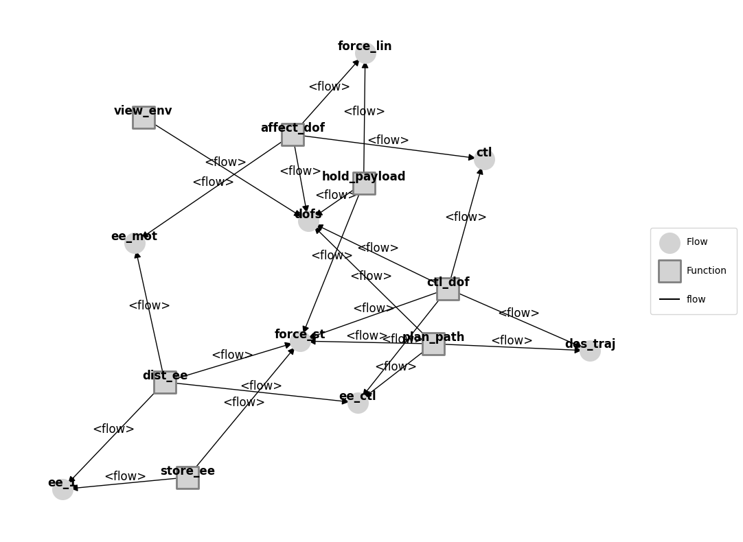
This graph is often pretty ugly by default because the layout is auto-generated via an algorithm in the networkx package
Making the graph pretty(er)
The outputted “Model Graph” is an Graph class (which heavily uses the networkx library), which has built-in options for applying different styles and moving nodes.
# %matplotlib qt5  # use this to have the graphs open up in an external window you can interact with
# mg.move_nodes() # this lets you move the nodes around in the external window
# %matplotlib inline  # this puts the matplotlib output back in the notebook
from model_static import pos
mg.set_pos(**pos)
mg.set_edge_labels(title="")
fig, ax = mg.draw(title="Graph of Drone Model Functions and Flows", withlegend=False, figsize=(5,5))
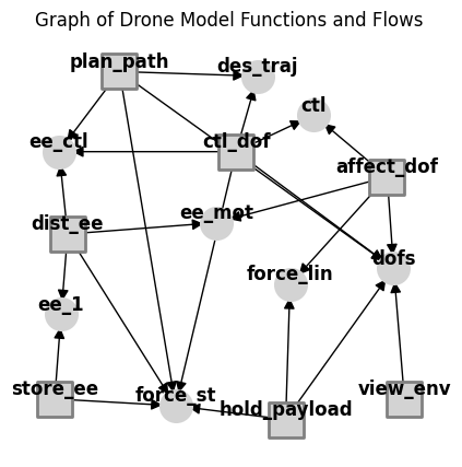
More info on working with graphs can be found in Tutorial: Model Structure Visualization
Simulation
There are several ways to simulate fmdtools models. One of the most flexible is to use the model directly:
mdl(0)
mdl
drone Drone
- t=Time(time=0.0, timers={})
- m=Mode(mode='nominal', faults=set(), sub_faults=False)
FLOWS:
- force_st=Force(s=(support=1.0))
- force_lin=Force(s=(support=1.0))
- ee_1=EE(s=(rate=1.0, effort=1.0))
- ee_mot=EE(s=(rate=1.0, effort=1.0))
- ee_ctl=EE(s=(rate=1.0, effort=1.0))
- ctl=Control(s=(forward=1.0, upward=1.0))
- dofs=DOFs(s=(vertvel=0.0, planvel=1.0, planpwr=1.0, uppwr=1.0, x=0.0, y=0.0, z=1.0))
- des_traj=DesTraj(s=(dx=1.0, dy=0.0, dz=0.0, power=1.0))
FXNS:
- store_ee=StoreEE(s=(soc=100.0), m=(mode='nominal', faults=set(), sub_faults=False))
- dist_ee=DistEE(s=(ee_tr=1.0, ee_te=1.0), m=(mode='nominal', faults=set(), sub_faults=False))
- affect_dof=AffectDOF(s=(e_to=1.0, e_ti=1.0, ct=1.0, mt=1.0, pt=1.0), m=(mode='nominal', faults=set(), sub_faults=False))
- ctl_dof=CtlDOF(s=(cs=1.0, power=1.0), m=(mode='nominal', faults=set(), sub_faults=False))
- plan_path=PlanPath(m=(mode='nominal', faults=set(), sub_faults=False))
- hold_payload=HoldPayload(s=(force_gr=0.0), m=(mode='nominal', faults=set(), sub_faults=False))
- view_env=ViewEnvironment(m=(mode='nominal', faults=set(), sub_faults=False))
Note the change in state in the system–most notably the incremented timestep (now 1).
Simulation Limitation
Since this model is only meant to run one timestep, simulating further gives us an error:
# mdl()
Simulation Parameter and History
Models can be run to different times depending on their Simulation Parameter (see: SimParam. The static model, by default, only simulates one timestep at t=0:
mdl.sp # simulation parameter
SimParam(phases=(('na', 0.0, 0),), start_time=0.0, end_time=0.0, track_times=('all',), dt=1.0, units='hr', end_condition='', use_local=True, with_loadings=False, run_stochastic=False, track_pdf=False)
This parameter can be changed at model instantiation and sets the end condition (in this case, end_time), which in turn determines how long the simulation will run and how long the history is. See:
mdl = Drone(sp={'end_time': 2})
mdl.h
time:                           array(3)
flows.force_st.s.support:       array(3)
flows.force_lin.s.support:      array(3)
flows.ee_1.s.rate:              array(3)
flows.ee_1.s.effort:            array(3)
flows.ee_mot.s.rate:            array(3)
flows.ee_mot.s.effort:          array(3)
flows.ee_ctl.s.rate:            array(3)
flows.ee_ctl.s.effort:          array(3)
flows.ctl.s.forward:            array(3)
flows.ctl.s.upward:             array(3)
flows.dofs.s.vertvel:           array(3)
flows.dofs.s.planvel:           array(3)
flows.dofs.s.planpwr:           array(3)
flows.dofs.s.uppwr:             array(3)
flows.dofs.s.x:                 array(3)
flows.dofs.s.y:                 array(3)
flows.dofs.s.z:                 array(3)
flows.des_traj.s.dx:            array(3)
flows.des_traj.s.dy:            array(3)
flows.des_traj.s.dz:            array(3)
flows.des_traj.s.power:         array(3)
fxns.store_ee.s.soc:            array(3)
fxns.store_ee.m.faults.nocharge: array(3)
fxns.store_ee.m.sub_faults:     array(3)
fxns.dist_ee.s.ee_tr:           array(3)
fxns.dist_ee.s.ee_te:           array(3)
fxns.dist_ee.m.faults.break:    array(3)
fxns.dist_ee.m.faults.degr:     array(3)
fxns.dist_ee.m.faults.short:    array(3)
fxns.dist_ee.m.sub_faults:      array(3)
fxns.affect_dof.s.e_to:         array(3)
fxns.affect_dof.s.e_ti:         array(3)
fxns.affect_dof.s.ct:           array(3)
fxns.affect_dof.s.mt:           array(3)
fxns.affect_dof.s.pt:           array(3)
fxns.affect_dof.m.faults.ctlbreak: array(3)
fxns.affect_dof.m.faults.ctldn: array(3)
fxns.affect_dof.m.faults.ctlup: array(3)
fxns.affect_dof.m.faults.mechbreak: array(3)
fxns.affect_dof.m.faults.mechfriction: array(3)
fxns.affect_dof.m.faults.openc: array(3)
fxns.affect_dof.m.faults.propbreak: array(3)
fxns.affect_dof.m.faults.propstuck: array(3)
fxns.affect_dof.m.faults.propwarp: array(3)
fxns.affect_dof.m.faults.short: array(3)
fxns.affect_dof.m.sub_faults:   array(3)
fxns.ctl_dof.s.cs:              array(3)
fxns.ctl_dof.s.power:           array(3)
fxns.ctl_dof.m.faults.degctl:   array(3)
fxns.ctl_dof.m.faults.noctl:    array(3)
fxns.ctl_dof.m.sub_faults:      array(3)
fxns.plan_path.m.faults.degloc: array(3)
fxns.plan_path.m.faults.noloc:  array(3)
fxns.plan_path.m.sub_faults:    array(3)
fxns.hold_payload.s.force_gr:   array(3)
fxns.hold_payload.m.faults.break: array(3)
fxns.hold_payload.m.faults.deform: array(3)
fxns.hold_payload.m.sub_faults: array(3)
fxns.view_env.m.sub_faults:     array(3)
Simulation: A more interesting case
To better showcase simulation, we are going to use the model in model_dynamic.py
This model builds on the architecture of the Drone model in model_static.py but adds behaviors that increment over time, meaning we can look at the behavior over multiple timesteps.
from model_dynamic import Drone

mdl = Drone()
mdl.sp
SimParam(phases=(('ascend', 0, 1), ('forward', 2, 14), ('descend', 15, 18), ('taxi', 19, 20)), start_time=0.0, end_time=20.0, track_times=('all',), dt=1.0, units='sec', end_condition='', use_local=True, with_loadings=False, run_stochastic=False, track_pdf=False)
A single timestep simulates via:
mdl()
mdl.t
Time(time=1.0, t_ind=1, timers={}, use_local=True, dt=1.0, executed_static=True, executed_dynamic=True, executing=False)
Or, to a given time-step:
mdl(time=20.0)
mdl.t
Time(time=20.0, t_ind=20, timers={}, use_local=True, dt=1.0, executed_static=True, executed_dynamic=True, executing=False)
Examining Simulation States
Given we’ve simulated the model to a given time-step, we can examine the states of the system and its history to see what happened:
mdl.fxns['store_ee'].s
StoreEEState(soc=89.5)
mdl.h.fxns.store_ee.s.soc
array([99.5, 99. , 98.5, 98. , 97.5, 97. , 96.5, 96. , 95.5, 95. , 94.5,
       94. , 93.5, 93. , 92.5, 92. , 91.5, 91. , 90.5, 90. , 89.5])
The classify method defined in the Model can also be used to classify the results of a given scenario.
from fmdtools.sim.scenario import Scenario
mdl.classify(scen=Scenario())
{'rate': 1.0, 'cost': 0, 'expected_cost': 0.0, 'lost_cost': 0, 'crashcost': 0}
We might want to be able to know more about the states of the system as a whole! We’ll cover more of that in the analysis portion of the tutorial.
Using the sim.propagate module
While you can always simulate models directly, sim.propagate has a lot of functionality that makes it easier to simulate scenarios of interest.
from fmdtools.sim import propagate
The simplest is propagate.nominal, which simulates the nominal scenario. Propagate methods return Result and History objects, like so:
res, hist = propagate.nominal(mdl)
res
tend.classify.rate:                  1.0
tend.classify.cost:                    0
tend.classify.expected_cost:         0.0
tend.classify.lost_cost:               0
tend.classify.crashcost:               0
hist
time:                          array(21)
flows.force_st.s.support:      array(21)
flows.force_lin.s.support:     array(21)
flows.ee_1.s.rate:             array(21)
flows.ee_1.s.effort:           array(21)
flows.ee_mot.s.rate:           array(21)
flows.ee_mot.s.effort:         array(21)
flows.ee_ctl.s.rate:           array(21)
flows.ee_ctl.s.effort:         array(21)
flows.ctl.s.forward:           array(21)
flows.ctl.s.upward:            array(21)
flows.dofs.s.vertvel:          array(21)
flows.dofs.s.planvel:          array(21)
flows.dofs.s.planpwr:          array(21)
flows.dofs.s.uppwr:            array(21)
flows.dofs.s.x:                array(21)
flows.dofs.s.y:                array(21)
flows.dofs.s.z:                array(21)
flows.des_traj.s.dx:           array(21)
flows.des_traj.s.dy:           array(21)
flows.des_traj.s.dz:           array(21)
flows.des_traj.s.power:        array(21)
flows.environment.c.r.probdens: array(21)
flows.environment.c.viewed:    array(21)
fxns.store_ee.s.soc:           array(21)
fxns.store_ee.m.faults.nocharge: array(21)
fxns.store_ee.m.sub_faults:    array(21)
fxns.dist_ee.s.ee_tr:          array(21)
fxns.dist_ee.s.ee_te:          array(21)
fxns.dist_ee.m.faults.break:   array(21)
fxns.dist_ee.m.faults.degr:    array(21)
fxns.dist_ee.m.faults.short:   array(21)
fxns.dist_ee.m.sub_faults:     array(21)
fxns.affect_dof.s.e_to:        array(21)
fxns.affect_dof.s.e_ti:        array(21)
fxns.affect_dof.s.ct:          array(21)
fxns.affect_dof.s.mt:          array(21)
fxns.affect_dof.s.pt:          array(21)
fxns.affect_dof.m.faults.ctlbreak: array(21)
fxns.affect_dof.m.faults.ctldn: array(21)
fxns.affect_dof.m.faults.ctlup: array(21)
fxns.affect_dof.m.faults.mechbreak: array(21)
fxns.affect_dof.m.faults.mechfriction: array(21)
fxns.affect_dof.m.faults.openc: array(21)
fxns.affect_dof.m.faults.propbreak: array(21)
fxns.affect_dof.m.faults.propstuck: array(21)
fxns.affect_dof.m.faults.propwarp: array(21)
fxns.affect_dof.m.faults.short: array(21)
fxns.affect_dof.m.sub_faults:  array(21)
fxns.ctl_dof.s.cs:             array(21)
fxns.ctl_dof.s.power:          array(21)
fxns.ctl_dof.m.faults.degctl:  array(21)
fxns.ctl_dof.m.faults.noctl:   array(21)
fxns.ctl_dof.m.sub_faults:     array(21)
fxns.plan_path.s.pt:           array(21)
fxns.plan_path.s.goal:         array(21)
fxns.plan_path.s.dist:         array(21)
fxns.plan_path.m.mode:         array(21)
fxns.plan_path.m.faults.degloc: array(21)
fxns.plan_path.m.faults.noloc: array(21)
fxns.plan_path.m.sub_faults:   array(21)
fxns.plan_path.t.pause.time:   array(21)
fxns.plan_path.t.pause.mode:   array(21)
fxns.hold_payload.s.force_gr:  array(21)
fxns.hold_payload.m.faults.break: array(21)
fxns.hold_payload.m.faults.deform: array(21)
fxns.hold_payload.m.sub_faults: array(21)
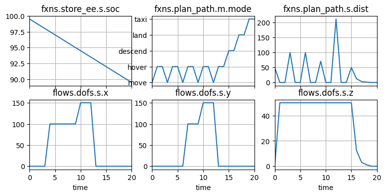
Verifying nominal outputs
With a history, you can use History.plot_line to verify that the system progresses through states as expected:
fig, axs = hist.plot_line("fxns.store_ee.s.soc", "fxns.plan_path.m.mode", "fxns.plan_path.s.dist", "flows.dofs.s.x", "flows.dofs.s.y", "flows.dofs.s.z", cols=3)
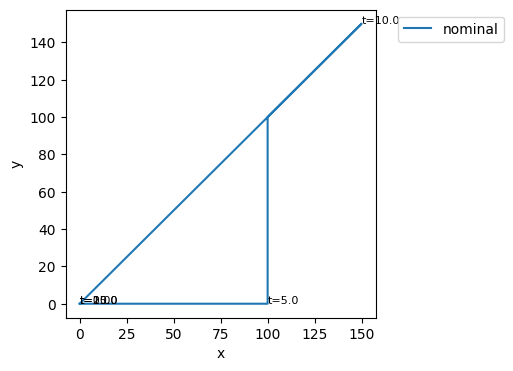
Verifying nominal trajectories
For trajectory information (x, y, and z coordinates), you can use History.plot_trajectories, which can work when there are two or three variables to plot:
# fix, ax = hist.plot_trajectories("flows.dofs.s.x", "flows.dofs.s.y", "flows.dofs.s.z", time_groups=["nominal"], time_ticks=5.0)
fix, ax = hist.plot_trajectories("flows.dofs.s.x", "flows.dofs.s.y", time_groups=["nominal"], time_ticks=5.0)
Simulating a fault scenario
We can simulate individual fault scenarios using propagate.one_fault. A fault scenario is a combination of a fault mode (defined as fault_faultname in a Mode) and a time.
Here we inject a nocharge fault into the store_ee function at time t=10.0:
res_lowcharge, hist_lowcharge = propagate.one_fault(mdl, "store_ee", "nocharge", 10.0)
res_lowcharge.faulty
tend.classify.rate:                1e-05
tend.classify.cost:             183000.0
tend.classify.expected_cost:    183000.0
tend.classify.lost_cost:           50000
tend.classify.crashcost:          100000
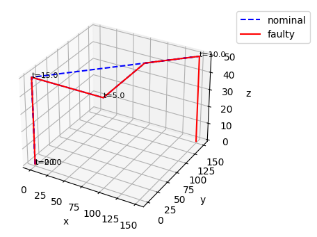
As shown, this causes a crash since the drone can no longer keep itself in the air:
fig, ax = hist_lowcharge.plot_trajectories("flows.dofs.s.x", "flows.dofs.s.y", "flows.dofs.s.z", time_groups=["nominal"], time_ticks=5.0)
Examining fault scenario results
When simulating scenarios, the returned Result and History objects include both nominal and faulty scenario information by default. This makes it easier to see what went wrong in a scenario, visualize scenarios and quantify metrics:
res_lowcharge.nest()
nominal:
--tend:
----classify:
------rate:                          1.0
------cost:                            0
------expected_cost:                 0.0
------lost_cost:                       0
------crashcost:                       0
store_ee_nocharge_t10p0:
--tend:
----classify:
------rate:                        1e-05
------cost:                     183000.0
------expected_cost:            183000.0
------lost_cost:                   50000
------crashcost:                  100000
We can get just the fault scenario results at .faulty
res_lowcharge.faulty
tend.classify.rate:                1e-05
tend.classify.cost:             183000.0
tend.classify.expected_cost:    183000.0
tend.classify.lost_cost:           50000
tend.classify.crashcost:          100000
Fault Graphs
Finally, we can use graphs to display the propagation of faults at any particular time by modifying the default to_return input parameter.
res_lowcharge, hist_lowcharge = propagate.one_fault(mdl, "store_ee", "nocharge", 10.0, to_return=['graph'])
res_lowcharge
nominal.tend.graph: <fmdtools.define.architecture.function.FunctionArchitectureGraph object at 0x000001530BE339D0>
store_ee_nocharge_t10p0.tend.graph: <fmdtools.define.architecture.function.FunctionArchitectureGraph object at 0x000001530BE33ED0>
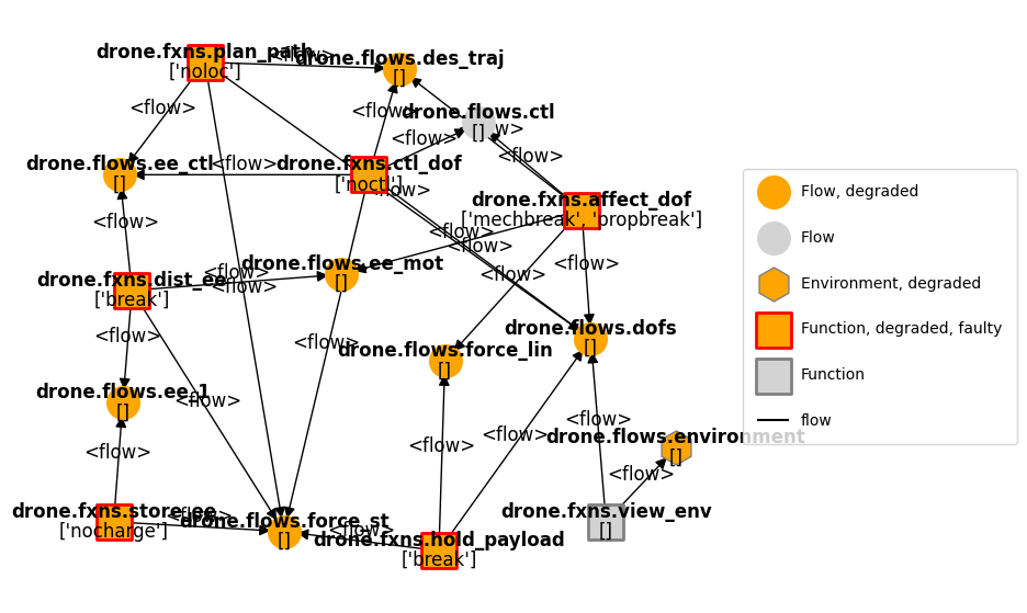
This graph shows degradations (blocks where the states deviate from the nominal state) in orange and faults (blocks where a fault mode has been entered) in red
res_lowcharge.faulty.tend.graph.set_pos(**pos, **{'drone.flows.environment':(1.0, -0.4)})
fig, ax = res_lowcharge.faulty.tend.graph.draw(figsize=(8,7))
More fault returns
We can get results from different times (rather than the end-time) by modifying the to_return argument further:
res_lowcharge, hist_lowcharge = propagate.one_fault(mdl, "store_ee", "nocharge", 10.0, to_return={10.0:['graph', 'classify'], "end": ['graph', 'classify']})
res_lowcharge
nominal.t10p0.classify.rate:         1.0
nominal.t10p0.classify.cost:      150000
nominal.t10p0.classify.expected_cost: 15000000000.0
nominal.t10p0.classify.lost_cost:  50000
nominal.t10p0.classify.crashcost: 100000
nominal.t10p0.graph: <fmdtools.define.architecture.function.FunctionArchitectureGraph object at 0x000001530BAC69E0>
nominal.tend.classify.rate:          1.0
nominal.tend.classify.cost:            0
nominal.tend.classify.expected_cost: 0.0
nominal.tend.classify.lost_cost:       0
nominal.tend.classify.crashcost:       0
nominal.tend.graph: <fmdtools.define.architecture.function.FunctionArchitectureGraph object at 0x000001530BAC76F0>
store_ee_nocharge_t1               1e-05
store_ee_nocharge_t1            150300.0
store_ee_nocharge_t1            150300.0
store_ee_nocharge_t1               50000
store_ee_nocharge_t1              100000
store_ee_nocharge_t10p0.t10p0.graph: <fmdtools.define.architecture.function.FunctionArchitectureGraph object at 0x000001530C4F8710>
store_ee_nocharge_t1               1e-05
store_ee_nocharge_t1            183000.0
store_ee_nocharge_t1            183000.0
store_ee_nocharge_t1               50000
store_ee_nocharge_t1              100000
store_ee_nocharge_t10p0.tend.graph: <fmdtools.define.architecture.function.FunctionArchitectureGraph object at 0x000001530BC05E10>
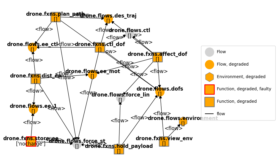
As shown on the graph, at t=10.0, when the fault is injected, not all of the faults have yet propagated:
res_lowcharge.faulty.t10p0.graph.set_pos(**pos, **{'drone.flows.environment':(1.0, -0.4)})
fig, ax = res_lowcharge.faulty.t10p0.graph.draw(figsize=(8,7))
More on single-scenario simulation
Simulation often can mean more than just simulating a fault, but can also include external disturbances or parameters. It may be helpful to familiarize yourself with the following methods:
propagate.sequencemethod: can be used to inject an arbitrary sequence of disturbances and faults in a model and simulate the resultspropagate.Simulationclass: gives more fine-grained control over event simulation, including model copying
As well as the options/parameters for these classes and methods.
propagate.sequence
<function fmdtools.sim.propagate.sequence(mdl, seq={}, faultseq={}, disturbances={}, scen={}, rate=nan, include_nominal=True, showprogress=False, **kwargs)>
help(propagate.Simulation)
Help on class Simulation in module fmdtools.sim.propagate:

class Simulation(BaseSimulation)
 |  Simulation(*args, **kwargs)
 |
 |  Simulate a single scenario.
 |
 |  Simulations can be used to do a few things, including:
 |  (1) Simulating a model in a particular faulty or nominal scenario
 |  (2) Getting model copies at particular times during a (usually nominal) scenario
 |  to simulate from. This is helpful for staged simulation where the copies are used
 |  to simulate faults from the point when the fault occurs instead of simulating
 |  up to that timestep first
 |  (3) Generating SampleApproaches that line up with the particular phases of the
 |  (usually nominal) scenario. This is helpful for nested simulations where each
 |  set of nominal parameters may change the phases of the simulation and thus the
 |  fault modes it may enter.
 |
 |  Parameters
 |  ----------
 |  scen : Scenario
 |      Scenario to simulation
 |  protect : bool
 |      Whether to protect the model by re-initializing it.
 |  copy : bool
 |      Whether to copy the model prior to simulation
 |  ctimes : list
 |      Times to copy the model from during simulation
 |  simevents : list
 |      SimEvents to run the system over. Generated from scenario, ctypes, etc.
 |  warn_faults : bool
 |      Whether to warn if the simulation is faulty and no faults were injected. Used
 |      for nominal simulations.
 |
 |  Examples
 |  --------
 |  >>> from fmdtools.define.block.function import ExampleFunction
 |  >>> sim = Simulation(mdl=ExampleFunction()) # default is nominal simulation
 |  >>> sim.name
 |  'nominal'
 |  >>> sim
 |  Simulation with SimEvents:
 |  - end=SimEvent(to_return={'classify': None})
 |  >>> res, hist = sim()
 |  >>> res
 |  tend.classify.xy:                  100.0
 |
 |  >>> esf = ExampleFunction() # here we try sometime more complicated:
 |  >>> s = SingleFaultScenario.from_fault(("examplefunction", "low"), 3.0, esf)
 |  >>> sim = Simulation(mdl=esf, scen=s, ctimes = [2, 4], to_return={1.0: 's.x', "end": ["classify", "graph"]})
 |  >>> sim
 |  Simulation with SimEvents:
 |  - 1.0=SimEvent(to_return={'s.x': None})
 |  - 2.0=SimEvent(copy=True)
 |  - 3.0=SimEvent(injection=Injection(faults={'examplefunction': ['low']}, disturbances={}))
 |  - 4.0=SimEvent(copy=True)
 |  - end=SimEvent(to_return={'classify': None, 'graph': None})
 |  >>> res, hist = sim()
 |  >>> sim.mdl
 |  examplefunction ExampleFunction
 |  - t=Time(time=100.0, timers={})
 |  - s=ExampleState(x=20.0, y=294.0)
 |  - m=ExampleMode(mode='low', faults={'low'}, sub_faults=False)
 |  - exf=ExampleFlow(s=(x=1964.0, y=1.0))
 |  >>> [*res.keys()]
 |  ['t1p0.s.x', 'tend.classify.xy', 'tend.graph']
 |  >>> sim.get_models()
 |  {2.0: examplefunction ExampleFunction
 |  - t=Time(time=1.0, timers={})
 |  - s=ExampleState(x=1.0, y=0.0)
 |  - m=ExampleMode(mode='standby', faults=set(), sub_faults=False)
 |  - exf=ExampleFlow(s=(x=2.0, y=1.0)), 4.0: examplefunction ExampleFunction
 |  - t=Time(time=3.0, timers={})
 |  - s=ExampleState(x=20.0, y=3.0)
 |  - m=ExampleMode(mode='low', faults={'low'}, sub_faults=False)
 |  - exf=ExampleFlow(s=(x=24.0, y=1.0))}
 |
 |  Method resolution order:
 |      Simulation
 |      BaseSimulation
 |      BaseSimContainer
 |      fmdtools.define.container.base.BaseContainer
 |      recordclass.datatype.dataobject
 |      builtins.object
 |
 |  Methods defined here:
 |
 |  __call__(self, with_mdls=False, gen_samp=False, **kwargs)
 |      Call the sim. Options return copied models and generated sampleapproches.
 |
 |  __init__(self, *args, **kwargs)
 |      Initialize and create the list of simulation events to run.
 |
 |  __repr__(self)
 |      Show event sequence in str.
 |
 |  check_faults(self)
 |      Check whether there are faults in a nominal simulation (a bad sign).
 |
 |  create_simevents(self)
 |      Create the list of SimEvents to run for during the simulation.
 |
 |  gen_sampleapproach(self, faultdomains={}, faultsamples={}, get_phasemap=False)
 |      Generate a SampleApproach from the simulation model.
 |
 |      Parameters
 |      ----------
 |      faultdomains : dict, optional
 |          dict of arguments to add_faultdomains. The default is {}.
 |      faultsamples : dict, optional
 |          dict of arguments to add_faultsamples. The default is {}.
 |      get_phasemap : bool, optional
 |          Whether to use the history to generate the phasemap used by SampleApproach.
 |          The default is False.
 |
 |      Returns
 |      -------
 |      app : SampleApproach
 |          Appropriate SampleApproach corresponding to this scenario model/hist
 |
 |  get_models(self)
 |      Get copied models from the simulation.
 |
 |  init_model(self)
 |      Initialize the model.
 |
 |      If self.protect, re-intiates the simulation with scenario parameters.
 |      If self.copy, copies the simulation.
 |
 |  run(self, **kwargs)
 |      Run the simevents and add results to the result dict.
 |
 |  ----------------------------------------------------------------------
 |  Data descriptors defined here:
 |
 |  __dict__
 |      dictionary for instance variables
 |
 |  copy
 |      Create an independent copy of the container with the same attributes.
 |
 |      Returns
 |      -------
 |      cop : BaseContainer
 |          Copy of the container with the same attributes as self.
 |      kwargs : kwargs
 |          Attributes of the container to overwrite with keyword arguments
 |
 |      Examples
 |      --------
 |      >>> ex = ExContainer(4.0, 5.0)
 |      >>> ex2 = ex.copy()
 |      >>> ex2
 |      ExContainer(x=4.0, y=5.0)
 |
 |      >>> ex_nest = ExNestContainer(ex2, 40.0)
 |      >>> ex_nest.copy(e1={'x': 6.0})
 |      ExNestContainer(e1=ExContainer(x=6.0, y=5.0), z=40.0)
 |
 |  ctimes
 |
 |  history
 |
 |  history_filename
 |
 |  indiv_id
 |
 |  mdl
 |
 |  name
 |
 |  overwrite
 |
 |  protect
 |
 |  result
 |
 |  result_filename
 |
 |  scen
 |
 |  simevents
 |
 |  to_return
 |
 |  tosave
 |
 |  warn_faults
 |
 |  ----------------------------------------------------------------------
 |  Data and other attributes defined here:
 |
 |  __annotations__ = {'copy': <class 'bool'>, 'ctimes': <class 'list'>, '...
 |
 |  __default_vals__ = ('', block Block
 |  - t=Time(time=-0.1, timers={}), {'...
 |
 |  __defaults__ = {'copy': False, 'ctimes': [], 'history': , 'history_fil...
 |
 |  __fields__ = ('name', 'mdl', 'to_return', 'tosave', 'overwrite', 'indi...
 |
 |  __match_args__ = ('name', 'mdl', 'to_return', 'tosave', 'overwrite', '...
 |
 |  __options__ = {'copy_default': True, 'fast_new': True, 'fields_dict': ...
 |
 |  ----------------------------------------------------------------------
 |  Methods inherited from BaseSimulation:
 |
 |  save(self)
 |      Save the results of the sim.
 |
 |  ----------------------------------------------------------------------
 |  Data descriptors inherited from BaseSimulation:
 |
 |  __weakref__
 |      list of weak references to the object
 |
 |  ----------------------------------------------------------------------
 |  Methods inherited from BaseSimContainer:
 |
 |  __setattr__(self, field, value)
 |      Revert to dataobject __setattr__.
 |
 |  ----------------------------------------------------------------------
 |  Methods inherited from fmdtools.define.container.base.BaseContainer:
 |
 |  asdict(self, *fields, jsonable=False, exclude=[], as_copy=False, **kwargs)
 |      Return fields as a dictionary.
 |
 |  assign(self, obj, *fields, as_copy=True, **fielddict)
 |      Set the same-named values of the current object to those of another.
 |
 |      Parameters
 |      ----------
 |      obj: Object/str/dict
 |          Object to assign values from
 |      *fields : fields to assign
 |      as_copy: bool,
 |          set to True for dicts/sets to be copied rather than referenced
 |      **fielddict : kwargs
 |          Mapping for arguments that don't match
 |
 |      Examples
 |      --------
 |      Further arguments specify which values. e.g.,:
 |
 |      >>> p1 = ExContainer(x=0.0, y=0.0)
 |      >>> p2 = ExContainer(x=10.0, y=20.0)
 |      >>> p1.assign(p2, 'x', 'y')
 |      >>> p1.x
 |      10.0
 |      >>> p1.y
 |      20.0
 |
 |      Can also be used to assign list values to a variable, e.g.,:
 |
 |      >>> p1.assign([3.0,4.0], 'x', 'y')
 |      >>> p1.x
 |      3.0
 |      >>> p1.y
 |      4.0
 |
 |      Can also provide kwargs in case value names don't match, e.g.,:
 |
 |      >>> p1.assign(p2, x='y', y='x')
 |      >>> p1.x
 |      20.0
 |      >>> p1.y
 |      10.0
 |
 |      Containers can also be assigned from json (including json files):
 |      >>> p1.assign('{"x": 1.0, "y": 2.0}', "x", "y")
 |      >>> p1
 |      ExContainer(x=1.0, y=2.0)
 |
 |  base_type(self)
 |      Return fmdtools type of the model class.
 |
 |  check_role(self, roletype, rolename)
 |      Check that the container will be given the correct name for its class.
 |
 |      The correct container-names correspond to the role for the class embody, e.g.:
 |          State : s
 |          Rand : r
 |          Mode : m
 |          Parameter : p
 |          SimParam : sp
 |
 |  create_hist(self, timerange=None, track=None, default_str_size='<U20')
 |      Create a History corresponding to the State.
 |
 |      Parameters
 |      ----------
 |      timerange : iterable, optional
 |          Time-range to initialize the history over. The default is None.
 |      track : list/str/dict, optional
 |          argument specifying attributes for :func:`get_sub_include'.
 |          The default is None.
 |
 |      Returns
 |      -------
 |      hist : History
 |          History of fields specified in track.
 |
 |      Examples
 |      --------
 |      >>> nest_hist = ExNestContainer().create_hist()
 |      >>> nest_hist
 |      e1:
 |      --x:                            array(1)
 |      --y:                            array(1)
 |      z:                              array(1)
 |      >>> nest_hist.e1.x
 |      [1.0]
 |
 |  create_repr(
 |      self,
 |      with_classname=True,
 |      fields=['all'],
 |      one_line=True,
 |      with_name=False
 |  )
 |      Create repr-friendly string for container.
 |
 |  get_code(self, source)
 |      Get the code defining the Container.
 |
 |  get_field_dict(self, obj, *fields, **fielddict)
 |      Get dict of values from object corresponding to Container fields.
 |
 |      Parameters
 |      ----------
 |      obj : dataobject, list, tuple, str (json or json filename) or ndarray
 |          Object to get field dictionary from.
 |      *fields : str
 |          Names of corresponding fields (in self.__fields__)
 |      **fielddict
 |          Mapping of fields in obj corresponding to fields in self.
 |
 |      Returns
 |      -------
 |      field_dict : dict
 |          Dictionary of fields and their values.
 |
 |      Examples
 |      --------
 |      >>> ex = ExContainer(1.0, 2.0)
 |      >>> ex.get_field_dict([5.0])
 |      {'x': 5.0}
 |
 |      >>> ex2 = ExContainer(3.0, 4.0)
 |      >>> ex.get_field_dict(ex2)
 |      {'x': 3.0, 'y': 4.0}
 |
 |      >>> ex.get_field_dict({'x': 3.0, 'z': 40.0}, x='x', y='z')
 |      {'x': 3.0, 'y': 40.0}
 |
 |      >>> ex.get_field_dict(ex)
 |      {'x': 1.0, 'y': 2.0}
 |
 |  get_fields(self, *fields, default='all')
 |      Get set of fields from the container.
 |
 |      Parameters
 |      ----------
 |      *fields : str
 |          Attributes to track. If 'all', gets all fields, if 'default', gets fields
 |          defined in self.default (where default is the name of default field list)
 |          if 'none', tracks none of the fields. if no fields provided, defaults to
 |          the default parameter.
 |
 |  get_memory(self)
 |      Get approximate memory impact of dataobject and its fields.
 |
 |  get_pref_attrs(self, prefix, space='_')
 |      Return dict of Container attributes with 'prefix_' as the var name.
 |
 |  get_track(self, track)
 |      Get tracking params for a given dataobject (State, Mode, Rand, etc).
 |
 |      Parameters
 |      ----------
 |      track : track
 |          str/tuple. Attributes to track.
 |          'all' tracks all fields
 |          'default' tracks fields defined in default_track for the dataobject
 |          'none' tracks none of the fields
 |
 |      Returns
 |      -------
 |      track : tuple
 |          fields to track
 |
 |  get_true_field(self, fieldname, *args, **kwargs)
 |      Get the value that will be set to fieldname given *args and **kwargs.
 |
 |  get_true_fields(self, *args, force_kwargs=False, **kwargs)
 |      Resolve the args to pass given certain defaults, *args and **kwargs.
 |
 |      NOTE: must be used for pickling, since pickle passes arguments as *args and not
 |      **kwargs.
 |
 |  get_typename(self)
 |      Containers are typed as containers unless specified otherwise.
 |
 |  init_hist_att(self, hist, att, timerange, track, str_size='<U20')
 |      Initialize a field in the history.
 |
 |  reset(self)
 |
 |  return_mutables(self)
 |      Return mutable aspects of the container.
 |
 |  set_arg_type(self, *args, **kwargs)
 |      Set Parameter field input to the predetermined field type.
 |
 |      e.g., if the input to parameter is int for a float field, this converts it to a
 |      float in initialization.
 |
 |      Parameters
 |      ----------
 |      *args : *args
 |          args to dataobject
 |      **kwargs : **kwargs
 |          kwargs to dataobject
 |
 |      Returns
 |      -------
 |      *new_args : tuple
 |          new args to dataobject (with proper type)
 |      **new_kwargs : dict
 |          new kwargs to dataobject (with proper type)
 |
 |  set_field(self, fieldname, value, as_copy=True)
 |      Set the field of the container to the given value.
 |
 |      Parameters
 |      ----------
 |      fieldname : str
 |          Name of the field.
 |      value : value
 |          Value to set the field to.
 |      as_copy : bool, optional
 |          Whether to copy value. The default is True.
 |
 |      Examples
 |      --------
 |      >>> ex_nest = ExNestContainer()
 |      >>> ex_inside = ExContainer(3.0, 4.0)
 |      >>> ex_nest.set_field('e1', ex_inside)
 |      >>> ex_nest
 |      ExNestContainer(e1=ExContainer(x=3.0, y=4.0), z=20.0)
 |
 |  to_default(self, *fieldnames)
 |      Reset given fields to their default values.
 |
 |      Examples
 |      --------
 |      >>> ex = ExContainer(3.0, 4.0)
 |      >>> ex.to_default()
 |      >>> ex
 |      ExContainer(x=1.0, y=2.0)
 |
 |      >>> ex = ExContainer(4.0, 5.0)
 |      >>> ex.to_default('x')
 |      >>> ex
 |      ExContainer(x=1.0, y=5.0)
 |
 |  tojson(self, fields=(), **mapping)
 |      Create json representation of current json values.
 |
 |  ----------------------------------------------------------------------
 |  Class methods inherited from fmdtools.define.container.base.BaseContainer:
 |
 |  fromdict(datadict, **mapping)
 |      Load from a dict.
 |
 |  fromjson(data, **mapping)
 |      Load from json string.
 |
 |  load(filename, delete=False, **mapping)
 |      Load values from file.
 |
 |  ----------------------------------------------------------------------
 |  Data and other attributes inherited from fmdtools.define.container.base.BaseContainer:
 |
 |  default_track = 'all'
 |
 |  rolename = 'x'
 |
 |  ----------------------------------------------------------------------
 |  Methods inherited from recordclass.datatype.dataobject:
 |
 |  __copy__(self, /)
 |      T.__copy__() -- copy of T
 |
 |  __eq__(self, value, /)
 |      Return self==value.
 |
 |  __ge__(self, value, /)
 |      Return self>=value.
 |
 |  __getstate__(self, /)
 |      T.__getstate__()
 |
 |  __gt__(self, value, /)
 |      Return self>value.
 |
 |  __hash__(self, /)
 |      Return hash(self).
 |
 |  __le__(self, value, /)
 |      Return self<=value.
 |
 |  __len__(self, /)
 |      Return len(self).
 |
 |  __lt__(self, value, /)
 |      Return self<value.
 |
 |  __ne__(self, value, /)
 |      Return self!=value.
 |
 |  __reduce__(self, /)
 |      T.__reduce__()
 |
 |  __setstate__(self, object, /)
 |      T.__setstate__()
 |
 |  __sizeof__(self, /)
 |      T.__sizeof__() -- size of T
 |
 |  ----------------------------------------------------------------------
 |  Static methods inherited from recordclass.datatype.dataobject:
 |
 |  __new__(*args, **kwargs) class method of recordclass.datatype.dataobject
 |      Create and return a new object.  See help(type) for accurate signature.
Simulating many scenarios
The propagate method has a few methods available to simulate ranges of nominal parameters, faulty scenarios, and disturbances. To get a feel for how this can be used, we can use propagate.single_faults, which simulates all single-fault scenarios possible in a model:
res_sf, hist_sf = propagate.single_faults(mdl, times=[5])
SCENARIOS COMPLETE: 100%|██████████| 20/20 [00:01<00:00, 12.06it/s]
As shown, this pulled 20 possible faults from the model and simulated them at the specified time (t=5). We can see the structure of the results below:
res_sf.nest()
nominal:
--tend:
----classify:
------rate:                          1.0
------cost:                            0
------expected_cost:                 0.0
------lost_cost:                       0
------crashcost:                       0
drone_fxns_store_ee_nocharge_t5:
--tend:
----classify:
------rate:                        1e-05
------cost:                     183000.0
------expected_cost:            183000.0
------lost_cost:                   50000
------crashcost:                  100000
drone_fxns_dist_ee_break_t5:
--tend:
----classify:
------rate:       2.0000000000000003e-06
------cost:                     182700.0
------expected_cost:   36540.00000000001
------lost_cost:                   50000
------crashcost:                  100000
drone_fxns_dist_ee_degr_t5:
--tend:
----classify:
------rate:                        5e-06
------cost:                     183700.0
------expected_cost:   91850.00000000001
------lost_cost:                   50000
------crashcost:                  100000
drone_fxns_dist_ee_short_t5:
--tend:
----classify:
------rate:                        3e-06
------cost:                     185700.0
------expected_cost:   55710.00000000001
------lost_cost:                   50000
------crashcost:                  100000
drone_fxns_affect_dof_ctlbreak_t5:
--tend:
----classify:
------rate:       2.0000000000000003e-06
------cost:                     183700.0
------expected_cost:   36740.00000000001
------lost_cost:                   50000
------crashcost:                  100000
drone_fxns_affect_dof_ctldn_t5:
--tend:
----classify:
------rate:       2.0000000000000003e-06
------cost:                     183200.0
------expected_cost:   36640.00000000001
------lost_cost:                   50000
------crashcost:                  100000
drone_fxns_affect_dof_ctlup_t5:
--tend:
----classify:
------rate:       2.0000000000000003e-06
------cost:                      50500.0
------expected_cost:  10100.000000000002
------lost_cost:                   50000
------crashcost:                       0
drone_fxns_affect_dof_mechbreak_t5:
--tend:
----classify:
------rate:       1.0000000000000002e-06
------cost:                     182700.0
------expected_cost:  18270.000000000004
------lost_cost:                   50000
------crashcost:                  100000
drone_fxns_affect_dof_mechfriction_t5:
--tend:
----classify:
------rate:        5.000000000000001e-07
------cost:                        500.0
------expected_cost:  25.000000000000007
------lost_cost:                       0
------crashcost:                       0
drone_fxns_affect_dof_openc_t5:
--tend:
----classify:
------rate:       1.0000000000000002e-06
------cost:                     182900.0
------expected_cost:  18290.000000000004
------lost_cost:                   50000
------crashcost:                  100000
drone_fxns_affect_dof_propbreak_t5:
--tend:
----classify:
------rate:       3.0000000000000004e-07
------cost:                     182700.0
------expected_cost:   5481.000000000001
------lost_cost:                   50000
------crashcost:                  100000
drone_fxns_affect_dof_propstuck_t5:
--tend:
----classify:
 ...168 lines
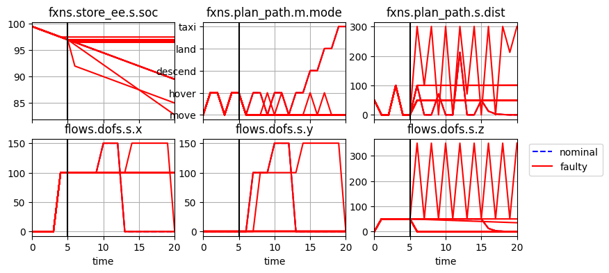
Visualizing many faults
We can use the same methods (plot_line and plot_trajectories) to visualize these results
fig, axs = hist_sf.plot_line("fxns.store_ee.s.soc", "fxns.plan_path.m.mode", "fxns.plan_path.s.dist", "flows.dofs.s.x", "flows.dofs.s.y", "flows.dofs.s.z", cols=3, time_slice=[5.0])
Grouping scenarios
While comparisons of nominal and faulty can be helpful, we can further separate groups based on the comp_groups parameter. Here we make each scenario its own group
fig, ax = hist_sf.plot_trajectories("flows.dofs.s.x", "flows.dofs.s.y", "flows.dofs.s.z", time_groups=["nominal"], comp_groups={k:k for k in hist_sf.nest()})
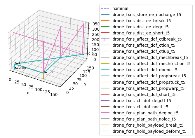
As shown, there are three main trajectories–crashing immediately (in grey), flying erratically (the ctlup fault in pink), and continuing the mission (in teal). Given this visualization, it may not be clear what scenarios ended in what outcome
More parameters can be used to visualize distributions of outcomes within these groups.
Aggregating results
Given this multi-scenario simulation, we can view tables of outcomes in aggregate:
tab = res_sf.create_simple_fmea()
tab.head(5) # showing an excerpt of the table
| rate | cost | expected_cost | lost_cost | crashcost | |
|---|---|---|---|---|---|
| nominal | 1.000000 | 0.0 | 0.0 | 0.0 | 0.0 |
| drone_fxns_store_ee_nocharge_t5 | 0.000010 | 183000.0 | 183000.0 | 50000.0 | 100000.0 |
| drone_fxns_dist_ee_break_t5 | 0.000002 | 182700.0 | 36540.0 | 50000.0 | 100000.0 |
| drone_fxns_dist_ee_degr_t5 | 0.000005 | 183700.0 | 91850.0 | 50000.0 | 100000.0 |
| drone_fxns_dist_ee_short_t5 | 0.000003 | 185700.0 | 55710.0 | 50000.0 | 100000.0 |
Since hazardous outcomes area each given costs, we can use this to get a better idea of which scenarios ended in a crash compared to not having an effect or causing the drone to fly erratically.
Specifying Scenarios to Simulate
To provide more control over what kinds of scenarios to simulate, fmdtools provides the sim.sample module. This module enables the definition of domains to sample scenarios from, as well as samples of the domain. The main classes provided are:
FaultDomain: Defines faults to sample from.FaultSample: Defines a set of fault scenarios over a given domain. May be simulated inpropagate.fault_sample.ParameterDomain: Defines a range of parameter(s) to sample from.ParameterSample: Defines a set of parameter values to simulate. May be simulated withpropagate.parameter_sampleSampleApproach: Defines a combination ofFaultSamples to be simulated over aParameterSample. May be simulated withpropagate.fault_sampleor constructed withpropagate.nested_sample
This tutorial will cover basic fault simulation. More materials are provided in Tutorial: FaultSample and Tutorial: ParameterSample
Defining a FaultDomain
We can define the set of faults to sample by first defining a fault domain:
from fmdtools.sim.sample import FaultDomain, FaultSample

fd = FaultDomain(mdl)
fd
FaultDomain with faults:
 -
For this we will need to add faults:
fd.add_fault("drone.fxns.store_ee", "nocharge")
fd.add_fault("drone.fxns.affect_dof", "ctlup")
fd
FaultDomain with faults:
 -('drone.fxns.store_ee', 'nocharge')
 -('drone.fxns.affect_dof', 'ctlup')
There are many more methods we can call from FaultDomain to add faults, including add_all (to add all possible fault modes) and add_all_fxn_modes (to add all modes from a given function)
Defining a FaultSample
FaultSamples define the set of fault scenarios to simulate based on these faults, given they could be simulated jointly or individually, as well as at different times.
fs = FaultSample(fd)
fs
FaultSample of scenarios:
 -
To add particular scenario times, we can use FaultSample.add_fault_times. FaultSample can also sample particular phases of operation (e.g., takeoff, flight, landing, taxi) statistically using numerical integration provided we give it this information via a PhaseMap using FaultSample.add_fault_phases.
fs.add_fault_times([5.0, 7.0, 15.0])
fs
FaultSample of scenarios:
 - drone_fxns_store_ee_nocharge_t5p0
 - drone_fxns_store_ee_nocharge_t7p0
 - drone_fxns_store_ee_nocharge_t15p0
 - drone_fxns_affect_dof_ctlup_t5p0
 - drone_fxns_affect_dof_ctlup_t7p0
 - drone_fxns_affect_dof_ctlup_t15p0
Simulating a FaultSample
This sample can in turn be simulated with propagate.fault_sample
res_fs, hist_fs = propagate.fault_sample(mdl, fs)
[*res_fs.nest(1)]
SCENARIOS COMPLETE: 100%|██████████| 6/6 [00:00<00:00, 6.31it/s]
['nominal',
 'drone_fxns_store_ee_nocharge_t5p0',
 'drone_fxns_store_ee_nocharge_t7p0',
 'drone_fxns_store_ee_nocharge_t15p0',
 'drone_fxns_affect_dof_ctlup_t5p0',
 'drone_fxns_affect_dof_ctlup_t7p0',
 'drone_fxns_affect_dof_ctlup_t15p0']
We can use the FaultSample to group and compare particular types of faults, for example:
comp_groups = {k[0]: v for k, v in fs.get_scen_groups("obj").items()}
comp_groups["nominal"] = ["nominal"]
comp_groups
{'drone.fxns.store_ee': ['drone_fxns_store_ee_nocharge_t5p0',
  'drone_fxns_store_ee_nocharge_t7p0',
  'drone_fxns_store_ee_nocharge_t15p0'],
 'drone.fxns.affect_dof': ['drone_fxns_affect_dof_ctlup_t5p0',
  'drone_fxns_affect_dof_ctlup_t7p0',
  'drone_fxns_affect_dof_ctlup_t15p0'],
 'nominal': ['nominal']}
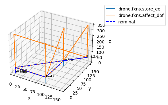
Visualizing Fault Groups
With particular fault groups defined, we can send them as comp_groups argument to various methods:
fig, ax = hist_fs.plot_trajectories("flows.dofs.s.x", "flows.dofs.s.y", "flows.dofs.s.z",
                                    comp_groups=comp_groups,
                                    time_groups=['nominal'], time_ticks=4.0)
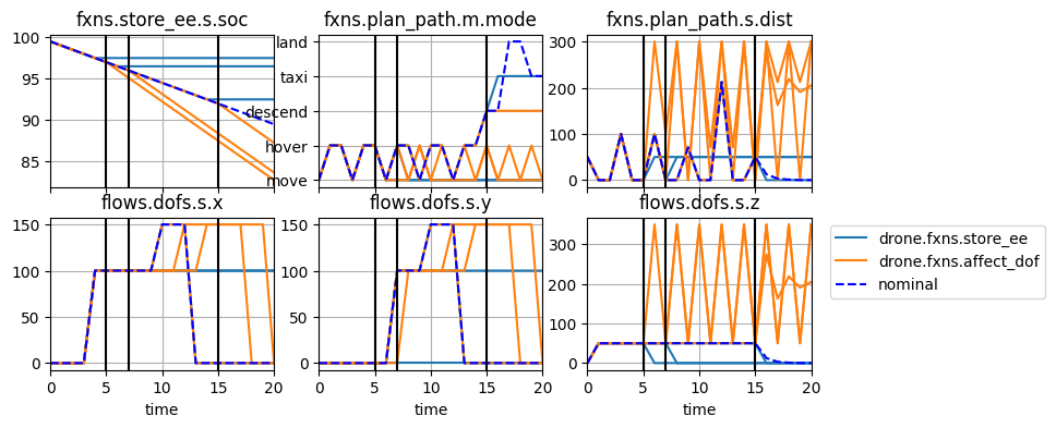
fig, axs = hist_fs.plot_line("fxns.store_ee.s.soc", "fxns.plan_path.m.mode", "fxns.plan_path.s.dist", "flows.dofs.s.x", "flows.dofs.s.y", "flows.dofs.s.z",
                             cols=3, comp_groups=comp_groups, time_slice=[5.0, 7.0, 15.0])
Tabular Comparison
FaultSample can also be used to group scenarios to help us make tables of fault simulation results, e.g., types of Failure Modes and Effects Analysis. See below:
from fmdtools.analyze.tabulate import FMEA, result_summary_fmea
fmeatab = FMEA(res_fs, fs)
fmeatab
<FMEA: 3 metric(s), 2 entries, metrics=['average_scenario_rate', 'sum_cost', 'expected_cost']>
By default, FMEA groups all results by function and mode.
fmeatab.as_table()
| average_scenario_rate | sum_cost | expected_cost | ||
|---|---|---|---|---|
| drone.fxns.store_ee | nocharge | 0.000007 | 499000.0 | 3.160 |
| drone.fxns.affect_dof | ctlup | 0.000001 | 151500.0 | 0.202 |
We can change how this is grouped, e.g.,
fmeatab = FMEA(res_fs, fs, group_by=("time", ))
fmeatab.as_table()
| average_scenario_rate | sum_cost | expected_cost | |
|---|---|---|---|
| 15.0 | 0.000006 | 183500.0 | 1.4310 |
| 7.0 | 0.000003 | 233500.0 | 0.9655 |
| 5.0 | 0.000003 | 233500.0 | 0.9655 |
How to Learn More
The best way to learn fmdtools is to try to build your own model. See if you can build something simple that uses some of the main fmdtools classes (
State,Mode,Function,FunctionArchitecture, etc.) and simulates in the way you want.It can help to look through the
/examples/folder to see what patterns we have used to model similar systemsWhen you are lost, or simply want to know how exactly to use a particular class or function, look at the [Module Reference](file:///C:/Users/dhulse/Documents/GitHub/fmdtools/docs/html/docs-source/fmdtools.html) for for that particular class. This same information is also available using Python’s built-in help function (e.g.
help(ClassName)).Finally, ask for help! Sometimes it can be quicker to ask someone who knows than to struggle on your own.