Paper [JMD]: Synthetic Mode Generation
For the paper Hulse, D., & Irshad, L. (2023). Synthetic fault mode generation for resilience analysis and failure mechanism discovery. Journal of mechanical design, 145(3), 031707.
This notebook shows how modes can be elaborated from health states in an fmdtools model.
Copyright © 2024, United States Government, as represented by the Administrator of the National Aeronautics and Space Administration. All rights reserved.

The “"Fault Model Design tools - fmdtools version 2"” software is licensed under the Apache License, Version 2.0 (the "License"); you may not use this file except in compliance with the License. You may obtain a copy of the License at http://www.apache.org/licenses/LICENSE-2.0.

Unless required by applicable law or agreed to in writing, software distributed under the License is distributed on an "AS IS" BASIS, WITHOUT WARRANTIES OR CONDITIONS OF ANY KIND, either express or implied. See the License for the specific language governing permissions and limitations under the License.
from fmdtools.sim.sample import FaultDomain, FaultSample
import fmdtools.sim.propagate as prop
import matplotlib.pyplot as plt
plt.rcParams['pdf.fonttype'] = 42
import multiprocessing as mp
import pandas as pd
import time
The Rover model is in defined model_main.py, along with a few analysis methods.
from fmdtools_examples.navigating_rover.model_main import Rover
Below we compare the space of hazards revealed by querying the model with:
identifed modes (modes that we identify up-front)
elaborated modes (modes generated by lists of forseeable parameter values)
randomly-generated modes (modes generated by randomly sampling ranges of parameter values)
from fmdtools.define.architecture.function import FunctionArchitectureFxnGraph
mdl_illust = Rover()
mg = FunctionArchitectureFxnGraph(mdl_illust)
fig, ax = mg.draw()
colors = ["goldenrod", "magenta", "blue"]
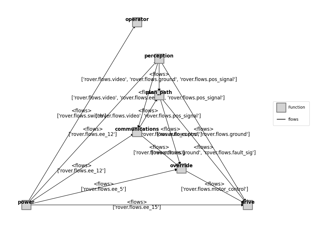
fig.savefig("outputs_paper_jmd_synthetic_modes/rover_structure.pdf", format="pdf", bbox_inches = 'tight', pad_inches = 0)
fig.savefig("outputs_paper_jmd_synthetic_modes/rover_structure.eps", format="eps", bbox_inches = 'tight', pad_inches = 0)
The PostScript backend does not support transparency; partially transparent artists will be rendered opaque.
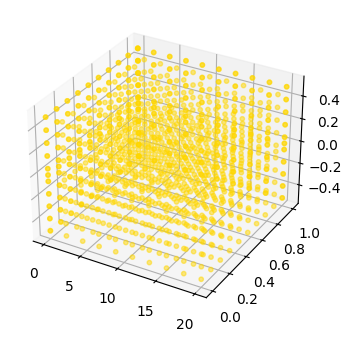
from fmdtools_examples.navigating_rover.script_mode_space import set_ranges, dist_ranges, p_test
mdl = Rover(p=p_test, sp={'end_condition': ''})
fd_range = FaultDomain(mdl)
fd_range.add_fault_space('drive', 'custom', dist_ranges)
from fmdtools.analyze.common import setup_plot
from mpl_toolkits.mplot3d import proj3d

def plot_labs(labs, x, y, z, fig):
    for i, label in enumerate(labs):
            xlab, ylab, _ = proj3d.proj_transform(x[i], y[i], z[i],  ax.get_proj())
            if label=='stuck_left':
                xyt=(-20,-30)
            elif label=='stuck':
                xyt=(20,-30)
            else:
                xyt=(20,30)
            plt.annotate(label, xy=(xlab, ylab), xytext=xyt,
                textcoords='offset points', ha='center', va='bottom',
                bbox=dict(boxstyle='round,pad=0.2', fc='white', alpha=1.0),
                arrowprops=dict(arrowstyle='-|>', color=colors[2]))

def plot_mode_space(faultdomain, size=30, alpha=0.5, label='', color='blue', marker='o', fig=None, ax=None, figsize=(4,4), show_labs=False):
    x = []
    y = []
    z = []
    labs = []
    for faulttup, fault in faultdomain.faults.items():
        dist_dict = dict(fault.disturbances)
        x.append(dist_dict.get('s.friction', 0.0))
        y.append(dist_dict.get('s.transfer', 1.0))
        z.append(dist_dict.get('s.drift', 0.0))
        labs.append(faulttup[1])

    fig, ax = setup_plot(fig=fig, ax=ax, figsize=figsize, z=True)
    ax.scatter(x, y, z, s=size, alpha=alpha, color=color, label=label, marker=marker)
    if show_labs:
        plot_labs(labs, x, y, z, fig)
    return fig, ax
fig, ax = plot_mode_space(fd_range, label='range', color='gold', size=10, alpha=0.5)
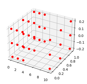
fd_set = FaultDomain(mdl)
fd_set.add_fault_space('drive', 'custom', set_ranges)
fig, ax = plot_mode_space(fd_set, color='red', alpha=1.0, label='set', size=30)
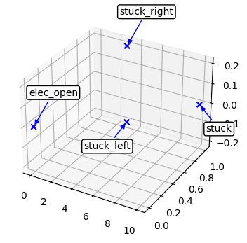
fd_id = FaultDomain(mdl)
fd_id.add_faults(('drive', 'stuck_right'), ('drive', 'stuck_left'), ('drive', 'stuck'), ('drive', 'elec_open'))
fig, ax = plot_mode_space(fd_id, color='blue', alpha=1.0, label='set', size=30, show_labs=True, marker='x')
def add_layer(fig, ax):
    proj=ax.get_tightbbox(fig.canvas.get_renderer())

    ax2 = fig.add_subplot(projection='3d')
    ax2.patch.set_alpha(0.0)
    xmin, ymin, zmin = proj3d.proj_transform(ax.get_xlim()[0], ax.get_ylim()[0], ax.get_zlim()[0],  ax.get_proj())
    xmax, ymax, zmax = proj3d.proj_transform(ax.get_xlim()[1], ax.get_ylim()[1], ax.get_zlim()[1],  ax.get_proj())
    ax2.set_xlim(xmin, xmax)
    ax2.set_ylim(ymin, ymax)
    ax2.set_zlim(zmin, zmax)
    plt.axis('off')
    return ax2


def plot_mode_spaces(fd_range, fd_set, fd_id, title="Space of Fault Modes"):
    fig, ax = plot_mode_space(fd_range, label='range', color='goldenrod', size=5, alpha=0.25)
    fig, ax = plot_mode_space(fd_set, color='magenta', alpha=0.25, label='set', size=30, fig=fig, ax=ax)
    fig, ax = plot_mode_space(fd_id, color='blue', alpha=1.0, label='set', size=30, marker='x', fig=fig, ax=ax)
    ax.scatter([0], [1], [0], label="nominal", marker="*", s=50)
    ax2 = add_layer(fig, ax)
    fig, ax2 = plot_mode_space(fd_id, color='blue', alpha=1.0, label='set', size=30, show_labs=True, marker='x', fig=fig, ax=ax2)

    ax.set_title(title)

    ax.set_xlabel('friction')
    ax.set_ylabel('transfer')
    ax.set_zlabel('drift')
    ax.legend()
    return fig, ax
Below we compare the space of fault modes generated by our identified sets:
fig, ax = plot_mode_spaces(fd_range, fd_set, fd_id)
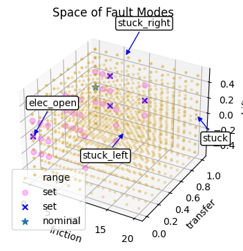
len(fd_range.faults)
1330
fig.savefig("outputs_paper_jmd_synthetic_modes/hazard_space.pdf", format="pdf", bbox_inches = 'tight', pad_inches = 0)
fig.savefig("outputs_paper_jmd_synthetic_modes/hazard_space.eps", format="eps", bbox_inches = 'tight', pad_inches = 0)
The PostScript backend does not support transparency; partially transparent artists will be rendered opaque.
fig.savefig("outputs_paper_jmd_synthetic_modes/hazard_space.svg", bbox_inches = 'tight', pad_inches = 0)
Analysis
Below we look at how this results in different potential analyses…
Finding phases so the Approach can inject the fault halfway through the simulation.
import fmdtools.analyze.phases as ph
endresults, mdlhist = prop.nominal(mdl)
phasemap = ph.from_hist(mdlhist)
endresults
tend.classify.rate:                  1.0
tend.classify.cost:                    0
tend.classify.prob:                  1.0
tend.classify.expected_cost:           0
tend.classify.in_bound:             True
tend.classify.at_finish:            True
tend.classify.line_dist:               1
tend.classify.num_modes:               0
tend.classify.end_dist:              0.0
tend.classify.tot_deviation: 0.005246344989065292
tend.classify.faults:           array(0)
tend.classify.classification: nominal mission
tend.classify.end_x:  29.813614084369863
tend.classify.end_y:   17.26588133276667
tend.classify.endpt:            array(2)
Simulating the set and range approach. Note that the identified modes are present in the range and mode approaches, so we end up taking this data from these results afterwards.
We simulate it here to get some idea of the simulation time.
t_id_0 = time.time()
fault_sample_id = FaultSample(fd_id, phasemap['plan_path'])
fault_sample_id.add_fault_phases('drive')
mdl = Rover(p=p_test, sp={'end_condition': ''})
results_id, mdlhists_id = prop.fault_sample(mdl, fault_sample_id, staged=True, pool=mp.Pool(5))
t_id = time.time()-t_id_0
t_id
SCENARIOS COMPLETE: 100%|██████████| 4/4 [00:02<00:00, 1.75it/s]
4.779683828353882
t_set_0 = time.time()
fs_set = FaultSample(fd_set, phasemap['plan_path'])
fs_set.add_fault_phases('drive')
results_set, mdlhists_set = prop.fault_sample(mdl, fs_set, staged=True,  pool=mp.Pool(5))
t_set = time.time() - t_set_0
t_set
SCENARIOS COMPLETE: 100%|██████████| 35/35 [00:03<00:00, 10.94it/s]
5.9383885860443115
t_range_0 = time.time()
fs_range = FaultSample(fd_range, phasemap['plan_path'])
fs_range.add_fault_phases('drive')
results_range, mdlhists_range = prop.fault_sample(mdl, fs_range, staged=True, pool=mp.Pool(5))
t_range = time.time() - t_range_0
t_range
SCENARIOS COMPLETE: 100%|██████████| 1330/1330 [01:12<00:00, 18.28it/s]
90.8149528503418
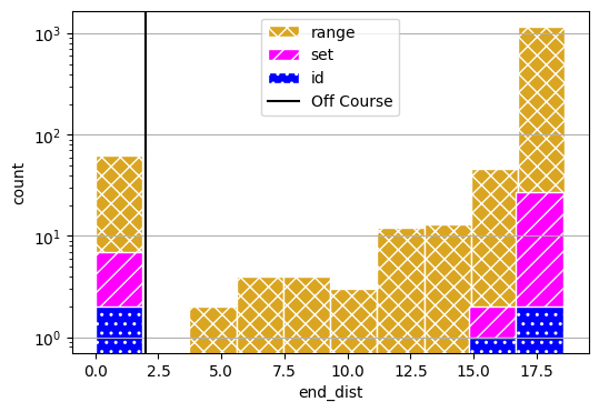
fig, axs = results_range.plot_metric_dist("end_dist", color=colors[0], hatch='xx', figsize=(6,4), edgecolor='white',
                                          comp_groups={'range': results_range.nest().keys()})
fig, axs = results_set.plot_metric_dist("end_dist", fig=fig, axs=axs, color=colors[1], hatch='//', edgecolor='white',
                                        comp_groups={'set': results_set.nest().keys()})
fig, axs = results_id.plot_metric_dist("end_dist", fig=fig, axs=axs, color=colors[2], hatch='..', edgecolor='white',
                                       comp_groups={'id': results_id.nest().keys()})
axs[0].axvline(2, label="Off Course", color="black")
axs[0].set_yscale("log")
axs[0].legend()
<matplotlib.legend.Legend at 0x284840b4550>
sim_times = [t_id, t_set, t_range]
sim_times
[4.779683828353882, 5.9383885860443115, 90.8149528503418]
fig.savefig("outputs_paper_jmd_synthetic_modes/line_dist.pdf", format="pdf", bbox_inches = 'tight', pad_inches = 0)
fig.savefig("outputs_paper_jmd_synthetic_modes/line_dist.eps", format="eps", bbox_inches = 'tight', pad_inches = 0)
The PostScript backend does not support transparency; partially transparent artists will be rendered opaque.
as well as the discovery of fault trajectories…
geoms = {'start': {'shapes': {'shape': {'color': 'black'}, 'near': {'color': 'grey', 'linestyle': 'dotted'}}},
        'end': {'shapes': {'shape': {'color': 'black'}, 'near': {'color': 'grey', 'linestyle': 'dotted'}}},
        'line': {'shapes': {'shape': {'color': 'black'}, 'near': {'color': 'grey', 'linestyle': 'dotted'}}}}

fig, ax = mdl.flows['ground'].ga.show(geoms, figsize = (8,8))

# comment out for tests/speed sake
fig, ax = mdlhists_range.plot_trajectories("flows.pos.s.x", "flows.pos.s.y",
                                        comp_groups = {'range': list(mdlhists_range.nest().keys())},
                                        fig=fig, ax=ax, color = colors[2])
fig, ax = mdlhists_set.plot_trajectories("flows.pos.s.x", "flows.pos.s.y",
                                         comp_groups = {'set': list(mdlhists_set.nest().keys())},
                                         color = colors[0], fig=fig, ax=ax)
fig, ax = mdlhists_id.plot_trajectories("flows.pos.s.x", "flows.pos.s.y",
                                        comp_groups = {'id': list(mdlhists_id.nest().keys())},
                                        fig=fig, ax=ax, color = colors[1])
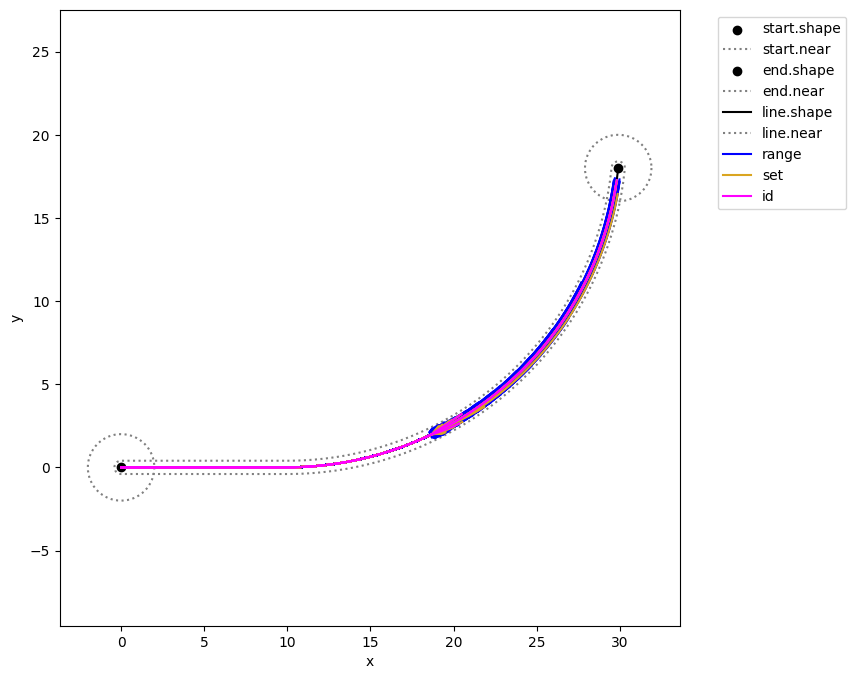
fig.savefig("outputs_paper_jmd_synthetic_modes/fault_map.pdf", format="pdf", bbox_inches = 'tight', pad_inches = 0)
fig.savefig("outputs_paper_jmd_synthetic_modes/fault_map.eps", format="eps", bbox_inches = 'tight', pad_inches = 0)
The PostScript backend does not support transparency; partially transparent artists will be rendered opaque.
fig.savefig("outputs_paper_jmd_synthetic_modes/fault_map.svg", bbox_inches = 'tight', pad_inches = 0)
Cluster Analysis
Below, we use clustering to identify similar sets of synthetic modes.
# import pip
# pip install scikit-learn
from sklearn.cluster import DBSCAN as cluster #DBSCAN
import numpy as np
def get_X(mdlhists, hmode = True):
    x = np.array([[value[-1]] for scen, value in mdlhists.get_values('flows.pos.s.x').items()])
    y = np.array([[value[-1]] for scen, value in mdlhists.get_values('flows.pos.s.y').items()])
    return np.concatenate((x, y), axis=1)
To find similar trajectories, we will cluster on the x-y coordinates of the end position of the Rover accross these scenarios:
X_range = get_X (mdlhists_range)
ec_range = [endclass for scen, endclass in results_range.get_values('end_dist').items() if scen[0:6]!='nominal']
X_set = get_X (mdlhists_set)
ec_set = [endclass for scen, endclass in results_set.get_values('end_dist').items() if scen[0:6]!='nominal']
X_id = get_X (mdlhists_id, hmode = False)
ec_id = [endclass for scen, endclass in results_id.get_values('end_dist').items() if scen[0:6]!='nominal']
To identify where all the clusters are accross all three approaches, we first have to combine the three sets of data into one (otherwise it might cluster differently).
X = np.concatenate((X_range, X_set, X_id))
This runs the clustering algorithm:
cl = cluster().fit(X)
labels = cl.labels_
The number of clusters is:
unique_labels = set(labels)
len(unique_labels)- (1 if -1 in labels else 0)
4
Here we plot the clusters on the course map to see what the algorithm identified.
fig=plt.figure()
mdl.flows['ground'].ga.show(geoms, figsize = (8,8))
#clust_colors = [plt.cm.Spectral(each) for each in np.linspace(0, 1, len(unique_labels))]
#clust_colors.reverse()
clust_colors = plt.cm.get_cmap('viridis', len(unique_labels)+1)
markers = ["+","*","x","^","."]

for i, k in enumerate(unique_labels):
    x_label = [x[0] for i,x in enumerate(X) if labels[i]==k]
    y_label = [x[1] for i,x in enumerate(X) if labels[i]==k]
    if k == -1: clust_lab = 'unclustered'
    else:       clust_lab = 'cluster '+str(k)
    plt.scatter(x_label, y_label, zorder=i, label=clust_lab, color=clust_colors.colors[i], marker=markers[i])

#plt.scatter(X_set[:,0],X_set[:,1], label='set', color='black', marker='+')

#plt.scatter(X_id[:,0],X_id[:,1], label='identified', color='gray', marker='X')

plt.grid()
plt.xlabel('x-distance (m)')
plt.ylabel('y-distance (m)')

plt.legend()
fig = plt.gcf()
C:\Users\dhulse\AppData\Local\Temp\1\ipykernel_33372\784500743.py:5: MatplotlibDeprecationWarning: The get_cmap function was deprecated in Matplotlib 3.7 and will be removed in 3.11. Use ``matplotlib.colormaps[name]`` or ``matplotlib.colormaps.get_cmap()`` or ``pyplot.get_cmap()`` instead.
  clust_colors = plt.cm.get_cmap('viridis', len(unique_labels)+1)
<Figure size 640x480 with 0 Axes>
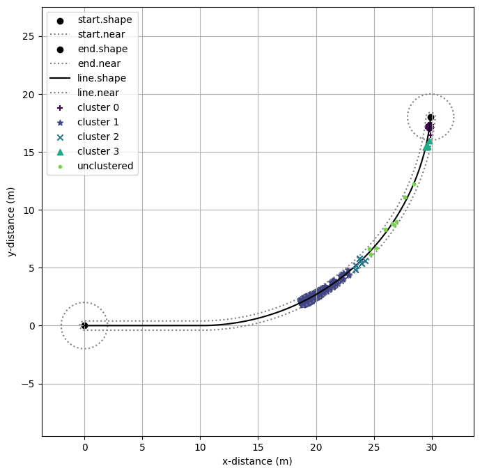
fig.savefig("outputs_paper_jmd_synthetic_modes/cluster_map.pdf", format="pdf", bbox_inches = 'tight', pad_inches = 0)
fig.savefig("outputs_paper_jmd_synthetic_modes/cluster_map.eps", format="eps", bbox_inches = 'tight', pad_inches = 0)
The PostScript backend does not support transparency; partially transparent artists will be rendered opaque.
Next, we would like to see how these approaches span the different clusters. If an approach has more coverage, we might say that it better explored the space.
categorizations = {tuple(x):labels[i] for i,x in enumerate(X)}
cat_values = {lab:{tuple(x) for x in X if lab==categorizations[tuple(x)]} for lab in set(labels)}
These are the categories found by each approach:
cat_range = [categorizations[tuple(x)] for x in X_range]
set(cat_range)
{np.int64(-1), np.int64(0), np.int64(1), np.int64(2), np.int64(3)}
cat_id = [categorizations[tuple(x)] for x in X_id]
set(cat_id)
{np.int64(0), np.int64(1)}
cat_set = [categorizations[tuple(x)] for x in X_set]
set(cat_set)
{np.int64(0), np.int64(1)}
ec_range
[0.0,
 18.212855187306467,
 17.880771586062338,
 12.97480547939998,
 17.304919376258646,
 18.15992894169864,
 9.465125171467097,
 17.072494800943055,
 17.63550537421338,
 17.92960283373589,
 17.926161520661,
 0.0,
 18.160411977987206,
 17.811098285415046,
 11.962856376045202,
 17.20021445899493,
 18.107972033888945,
 6.247923520595959,
 16.969489245356648,
 17.565909538279886,
 17.87580779695436,
 17.870028982816798,
 0.0,
 18.418450040639797,
 18.122472072307584,
 15.07168003139923,
 17.680999749424487,
 18.346533397417247,
 14.42565200789203,
 17.670554639726387,
 17.879888083653377,
 18.124189825231365,
 18.15065986239579,
 0.0,
 18.329590688049468,
 18.035205134978295,
 14.37113351947878,
 17.5430508824882,
 18.271455741177522,
 12.666149833487385,
 17.306929761613873,
 17.79099884406752,
 18.04763120305605,
 18.052212035287646,
 0.0,
 18.267454082042264,
 17.95509328259392,
 13.67247110611889,
 17.41852729995098,
 18.21430531405481,
 11.536024855214608,
 17.184299991893926,
 17.710112335390008,
 17.98659895519117,
 17.98594106232316,
 0.0,
 18.501403118868254,
 18.251999147059095,
 15.775299363087274,
 17.835782207472718,
 18.436102420934056,
 15.380597677113293,
 17.793896358667457,
 18.00120039935969,
 18.222840102055603,
 18.257519319356998,
 1.6193825180753854,
 18.60417775203917,
 18.41185862771426,
 16.4840067738236,
 18.163478754526384,
 18.526478540557985,
 16.27634672637296,
 17.9529372610547,
 18.16946360424912,
 18.25268512129733,
 18.371722052083015,
 4.9482796992796345,
 18.5708843523618,
 18.554756575850135,
 17.201282469904108,
 18.398118051108085,
 18.599507593422135,
 17.10504791208172,
 18.187213008779068,
 18.321602494550763,
 18.381693187650896,
 18.36691300655526,
 8.810318698943334,
 18.577729888050552,
 18.55771205798935,
 18.218008079921667,
 18.621224910607744,
 18.58280888450569,
 18.058968165621604,
 18.417160819334917,
 18.34256686044713,
 18.38234258439277,
 18.40086561208814,
 13.320276652456167,
 18.536161858187022,
 18.536161858187022,
 18.536161858187022,
 18.536161858187022,
 18.536161858187022,
 18.536161858187022,
 18.536161858187022,
 18.536161858187022,
 18.536161858187022,
 18.536161858187022,
 18.536161858187022,
 18.160411977987206,
 17.811098285415046,
 11.962856376045202,
 17.20021445899493,
 18.107972033888945,
 6.247923520595959,
 16.969489245356648,
 17.565909538279886,
 17.87580779695436,
 17.870028982816798,
 0.0,
 18.260857849134442,
 17.87625099453106,
 0.0,
 16.80170823614398,
 17.986619815051387,
 0.0,
 16.24852751223232,
 17.650354113761697,
 18.000496320187207,
 18.016688753902613,
 0.0,
 18.192438993994134,
 17.756771963200613,
 0.0,
 16.25210881866716,
 17.867030214206025,
 0.0,
 15.661561034936566,
 17.16228065852638,
 17.565156269441253,
 17.946413876924577,
 0.0,
 18.457290590487194,
 18.23489252680239,
 16.285624457261484,
 17.961490943747993,
 18.336072855284055,
 14.60561656808208,
 17.736906410942428,
 17.996061248264507,
 18.04747959652674,
 18.24659244336268,
 0.0,
 18.394490208377505,
 18.116170664228743,
 0.0,
 17.789777081659295,
 18.222861637851526,
 0.0,
 17.57867445456135,
 17.874336926023922,
 18.14303339464949,
 18.16655852891428,
 0.0,
 18.328504659621625,
 17.996260466927254,
 0.0,
 17.34855055008068,
 18.105636945598825,
 0.0,
 16.800441177960668,
 17.75947096221344,
 18.070102103521016,
 18.089971720140074,
 0.0,
 18.513250199963025,
 18.350118739368057,
 17.316810394929444,
 18.131503970725635,
 18.44105720015659,
 16.909212875746547,
 17.904821358126302,
 18.12572561924348,
 18.185732839107022,
 18.250919899230308,
 1.0449951885291886,
 18.59107926280268,
 18.431665838127767,
 17.686551106492928,
 18.29714740138886,
 18.52843358549255,
 17.595091354306522,
 18.08459980772958,
 18.26426563586251,
 18.330120857995713,
 18.368087511016952,
 14.957088713425764,
 18.531425425092664,
 18.54712288118584,
 18.04581003962738,
 18.4283752223622,
 18.602894999396156,
 17.824121181126934,
 18.21339463341425,
 18.345535041325768,
 18.36863206818473,
 18.304726137484682,
 15.803898027152883,
 18.584173070801942,
 18.560124756742205,
 18.344862416766727,
 18.60662441506524,
 18.567897537385246,
 18.140973528000565,
 18.40847814161987,
 18.37446250101867,
 18.36076225909854,
 18.386558518133974,
 15.922627204831166,
 18.536161858187022,
 18.536161858187022,
 18.536161858187022,
 18.536161858187022,
 18.536161858187022,
 18.536161858187022,
 18.536161858187022,
 18.536161858187022,
 18.536161858187022,
 18.536161858187022,
 18.536161858187022,
 18.192438993994134,
 17.756771963200613,
 0.0,
 16.25210881866716,
 17.867030214206025,
 0.0,
 15.661561034936566,
 17.16228065852638,
 17.565156269441253,
 17.946413876924577,
 0.0,
 18.19310683865107,
 17.815885950637536,
 0.0,
 17.191259031720072,
 18.109193186314442,
 0.0,
 16.66138003809095,
 17.54808882664952,
 17.847705984828657,
 18.121462363520603,
 0.0,
 18.266514330693944,
 17.68011303605772,
 0.0,
 16.67692201515722,
 18.014941537733417,
 0.0,
 15.491442768650398,
 17.426561003534808,
 17.756388883217827,
 18.06439463619541,
 0.0,
 18.451018321930036,
 18.216772506455687,
 17.141908104044134,
 17.967551914395937,
 18.382514800914524,
 16.73036122395024,
 17.719472851254444,
 18.105713904385663,
 18.148680614061316,
 18.197527480308892,
 11.21934208029755,
 18.370542471874536,
 18.209898536965703,
 16.178583536013164,
 17.79319863187439,
 18.294334937778267,
 14.789558422255121,
 17.551483241004103,
 18.00670943942227,
 18.043367505610387,
 18.087307184273506,
 0.0,
 18.28365279457688,
 17.95128159595894,
 12.607880526580965,
 17.617191237642377,
 18.202668143338897,
 0.0,
 17.391100748626336,
 17.912787823601423,
 17.94317221784124,
 18.180772654098604,
 0.0,
 18.519156369169743,
 18.34271223974877,
 17.598720907056823,
 18.138927920181516,
 18.46372230909453,
 17.38448890480213,
 17.896152400329147,
 18.095675234987905,
 18.259372631636907,
 18.31139608351588,
 15.081656743783713,
 18.591830365298513,
 18.456963810350853,
 17.884367573412867,
 18.304117130647857,
 18.530973090478515,
 17.670625377266063,
 18.083008184909875,
 18.251502777664644,
 18.329785786933506,
 18.384978035186084,
 15.747621217618027,
 18.55414676078107,
 18.549422046277808,
 18.112151434440772,
 18.437807956665036,
 18.606665641635445,
 17.896756965351173,
 18.230576620213768,
 18.334735832347775,
 18.401443900033104,
 18.349049806455046,
 15.879096613416806,
 18.58299319392777,
 18.55202667135574,
 18.34547945436056,
 18.60812063414016,
 18.56620043292363,
 18.161136317686093,
 18.410756958798878,
 18.37265647277308,
 18.360503771080598,
 18.393755565922085,
 15.896773927724045,
 18.536161858187022,
 18.536161858187022,
 18.536161858187022,
 18.536161858187022,
 18.536161858187022,
 18.536161858187022,
 18.536161858187022,
 18.536161858187022,
 18.536161858187022,
 18.536161858187022,
 18.536161858187022,
 18.266514330693944,
 17.68011303605772,
 0.0,
 16.67692201515722,
 18.014941537733417,
 0.0,
 15.491442768650398,
 17.426561003534808,
 17.756388883217827,
 18.06439463619541,
 0.0,
 18.255613867724698,
 17.94618450284477,
 0.0,
 17.43613561074165,
 18.186011122226905,
 0.0,
 16.976577128341248,
 17.71446025521068,
 17.964248484571627,
 17.99266154062866,
 0.0,
 18.179321690698142,
 17.83416169505078,
 0.0,
 17.01615903706855,
 18.108188983583474,
 0.0,
 16.25499128048522,
 17.612250096308944,
 17.88772415836104,
 17.911977286793928,
 0.0,
 18.467360432274667,
 18.27580580217769,
 17.263873546883936,
 18.071915767200405,
 18.36793556469948,
 17.036227705813396,
 17.858369552997562,
 18.048864841215288,
 18.215523222676836,
 18.256329256538148,
 14.331236006242543,
 18.401463142178972,
 18.167914762191508,
 16.78485654516362,
 17.928648249715614,
 18.338545213148013,
 16.188675864097874,
 17.717863955259443,
 17.932074221023917,
 18.12775123931038,
 18.164715761639822,
 1.5129309265167745,
 18.330083399712652,
 18.057606039145696,
 15.403305729684186,
 17.615939281502403,
 18.26303963174751,
 9.476212061413252,
 17.374624960354545,
 17.820805478824333,
 18.04414237421781,
 18.07685361703064,
 0.0,
 18.521766648124686,
 18.378990308004283,
 17.670154211220304,
 18.212418272955134,
 18.459829904285115,
 17.45404443083078,
 18.005807221642083,
 18.171841180372464,
 18.23419215953081,
 18.29892898812163,
 15.459870904063346,
 18.60245934205639,
 18.456674971320155,
 17.935386646061538,
 18.30773080565512,
 18.533020264004165,
 17.72467070228519,
 18.08313698884621,
 18.243276447284988,
 18.329657714927762,
 18.396003850788524,
 15.878267918511698,
 18.540615824318692,
 18.549712902567734,
 18.151607266722664,
 18.443288244726407,
 18.58483464249903,
 17.946260817938185,
 18.241878897972285,
 18.348803121875232,
 18.383511810446176,
 18.325639344509874,
 15.92374910806055,
 18.570659384671366,
 18.555387156959803,
 18.35730060858411,
 18.609085548071743,
 18.568207801572033,
 18.174473600131023,
 18.412245322437517,
 18.36946145828139,
 18.36357287377023,
 18.36659090700077,
 15.938427161620968,
 18.536161858187022,
 18.536161858187022,
 18.536161858187022,
 18.536161858187022,
 18.536161858187022,
 18.536161858187022,
 18.536161858187022,
 18.536161858187022,
 18.536161858187022,
 18.536161858187022,
 18.536161858187022,
 18.179321690698142,
 17.83416169505078,
 0.0,
 17.01615903706855,
 18.108188983583474,
 0.0,
 16.25499128048522,
 17.612250096308944,
 17.88772415836104,
 17.911977286793928,
 0.0,
 18.212855187306467,
 17.880771586062338,
 12.97480547939998,
 17.304919376258646,
 18.15992894169864,
 9.465125171467097,
 17.072494800943055,
 17.63550537421338,
 17.92960283373589,
 17.926161520661,
 0.0,
 18.160411977987206,
 17.811098285415046,
 11.962856376045202,
 17.20021445899493,
 18.107972033888945,
 6.247923520595959,
 16.969489245356648,
 17.565909538279886,
 17.87580779695436,
 17.870028982816798,
 0.0,
 18.418450040639797,
 18.122472072307584,
 15.07168003139923,
 17.680999749424487,
 18.346533397417247,
 14.42565200789203,
 17.670554639726387,
 17.879888083653377,
 18.124189825231365,
 18.15065986239579,
 0.0,
 18.329590688049468,
 18.035205134978295,
 14.37113351947878,
 17.5430508824882,
 18.271455741177522,
 12.666149833487385,
 17.306929761613873,
 17.79099884406752,
 18.04763120305605,
 18.052212035287646,
 0.0,
 18.267454082042264,
 17.95509328259392,
 13.67247110611889,
 17.41852729995098,
 18.21430531405481,
 11.536024855214608,
 17.184299991893926,
 17.710112335390008,
 17.98659895519117,
 17.98594106232316,
 0.0,
 18.501403118868254,
 18.251999147059095,
 15.775299363087274,
 17.835782207472718,
 18.436102420934056,
 15.380597677113293,
 17.793896358667457,
 18.00120039935969,
 18.222840102055603,
 18.257519319356998,
 1.6193825180753854,
 18.60417775203917,
 18.41185862771426,
 16.4840067738236,
 18.163478754526384,
 18.526478540557985,
 16.27634672637296,
 17.9529372610547,
 18.16946360424912,
 18.25268512129733,
 18.371722052083015,
 4.9482796992796345,
 18.5708843523618,
 18.554756575850135,
 17.201282469904108,
 18.398118051108085,
 18.599507593422135,
 17.10504791208172,
 18.187213008779068,
 18.321602494550763,
 18.381693187650896,
 18.36691300655526,
 8.810318698943334,
 18.577729888050552,
 18.55771205798935,
 18.218008079921667,
 18.621224910607744,
 18.58280888450569,
 18.058968165621604,
 18.417160819334917,
 18.34256686044713,
 18.38234258439277,
 18.40086561208814,
 13.320276652456167,
 18.536161858187022,
 18.536161858187022,
 18.536161858187022,
 18.536161858187022,
 18.536161858187022,
 18.536161858187022,
 18.536161858187022,
 18.536161858187022,
 18.536161858187022,
 18.536161858187022,
 18.536161858187022,
 18.160411977987206,
 17.811098285415046,
 11.962856376045202,
 17.20021445899493,
 18.107972033888945,
 6.247923520595959,
 16.969489245356648,
 17.565909538279886,
 17.87580779695436,
 17.870028982816798,
 18.298577087627095,
 17.89358960506939,
 8.813866561093423,
 17.432550627913656,
 18.12503681664753,
 0.0,
 17.202978254762932,
 17.833671664072146,
 17.86411112778984,
 18.07212523097011,
 0.0,
 18.233680018258486,
 17.769229156774333,
 0.0,
 17.04618939396206,
 18.030550535085155,
 0.0,
 16.587086745373185,
 17.525023892137856,
 17.771016027108445,
 18.002906014995457,
 0.0,
 18.461315455181836,
 18.256786432827788,
 17.34701535438947,
 18.058268566834524,
 18.39466840120688,
 17.1211074431062,
 17.83302847792131,
 18.120446201756145,
 18.168539560054658,
 18.222032054695816,
 14.8476171866188,
 18.422568146066805,
 18.224558524368362,
 16.91276042055952,
 17.90890885316047,
 18.30866452262992,
 16.532169036965332,
 17.685309615270356,
 18.02041072083577,
 18.0625139308383,
 18.219436189824968,
 8.524457144548327,
 18.36192981599624,
 18.13081440747535,
 15.890879763513572,
 17.757374561907387,
 18.218174503560228,
 13.954835650971216,
 17.54345355431865,
 17.924977295901936,
 17.96115174006938,
 18.144210162500784,
 1.5744472911676741,
 18.52344726522859,
 18.369107297295884,
 17.718688788033504,
 18.204227036403175,
 18.45685994650775,
 17.504950213291878,
 17.987626269284036,
 18.145107174687553,
 18.27903507376564,
 18.33429080280827,
 15.615801630934337,
 18.601286851877514,
 18.45633088398244,
 17.969862762134042,
 18.309950867300543,
 18.534601536317727,
 17.763791313073774,
 18.15012789177114,
 18.237512595758787,
 18.32936632351683,
 18.39066527475649,
 15.892288130293624,
 18.5600078105701,
 18.551185160113,
 18.144541439971672,
 18.435166976213075,
 18.586958434823597,
 17.981590608164744,
 18.249853320051134,
 18.3590461655547,
 18.374000762943382,
 18.333059379343425,
 15.905433413854244,
 18.577372496454515,
 18.55051694864354,
 18.365152050697933,
 18.609752320784988,
 18.563078635978165,
 18.183892755345845,
 18.413299630636043,
 18.367777780556853,
 18.36739686048938,
 18.374321850814006,
 16.317777025144935,
 18.536161858187022,
 18.536161858187022,
 18.536161858187022,
 18.536161858187022,
 18.536161858187022,
 18.536161858187022,
 18.536161858187022,
 18.536161858187022,
 18.536161858187022,
 18.536161858187022,
 18.536161858187022,
 18.233680018258486,
 17.769229156774333,
 0.0,
 17.04618939396206,
 18.030550535085155,
 0.0,
 16.587086745373185,
 17.525023892137856,
 17.771016027108445,
 18.002906014995457,
 0.0,
 18.481688582231826,
 18.46427105671697,
 18.44837828749458,
 18.4559001612946,
 18.473010617196785,
 18.44213276466692,
 18.437432521791266,
 18.434333396012676,
 18.4326981136084,
 18.43226877929391,
 18.445074463126257,
 18.470062808111873,
 18.452625668147615,
 18.43698521865384,
 18.444392784254035,
 18.461303146667017,
 18.430733064260494,
 18.425850316672257,
 18.4223999355376,
 18.420301908136068,
 18.419374810228586,
 18.433698006409244,
 18.51518459945436,
 18.499369764213796,
 18.482611510579442,
 18.490652702108743,
 18.507737286786114,
 18.47639723358406,
 18.47266772320141,
 18.471280444741307,
 18.47158086102681,
 18.47286044487028,
 18.479216573603065,
 18.504432491172416,
 18.487663849910113,
 18.471188240609894,
 18.479020132533016,
 18.496323116812178,
 18.46496038640355,
 18.460803517433387,
 18.458699694190628,
 18.458260445057274,
 18.45896886522497,
 18.46783375065413,
 18.493188339343707,
 18.47595309746492,
 18.45977851414564,
 18.467439559208568,
 18.484703844439146,
 18.453540814730193,
 18.44907434758331,
 18.44641368781603,
 18.445327597397256,
 18.445449506970036,
 18.456453045852488,
 18.525020618169435,
 18.510963613330077,
 18.49405590139688,
 18.502343673806006,
 18.51866087389929,
 18.48786294636763,
 18.48475438351301,
 18.484286617968632,
 18.485363987400508,
 18.487088793670136,
 18.490601510772734,
 18.533214658072403,
 18.522122930135918,
 18.50553717432087,
 18.514060512369362,
 18.528484380895346,
 18.499384655173433,
 18.497233352940597,
 18.49787893311276,
 18.499585584361732,
 18.501435498759392,
 18.50198855822588,
 18.53865066145183,
 18.53190567941041,
 18.51709193371393,
 18.525538094401433,
 18.53599428423821,
 18.5110425132047,
 18.51042762760607,
 18.512085029425126,
 18.513857303661755,
 18.515294014573396,
 18.513377711965635,
 18.539962786963983,
 18.537884922129134,
 18.52877606630761,
 18.535152439115198,
 18.539207023634315,
 18.523186330067546,
 18.524576443679752,
 18.526015938699565,
 18.52689015301727,
 18.527446445444316,
 18.524768967594508,
 18.536161858187022,
 18.536161858187022,
 18.536161858187022,
 18.536161858187022,
 18.536161858187022,
 18.536161858187022,
 18.536161858187022,
 18.536161858187022,
 18.536161858187022,
 18.536161858187022,
 18.536161858187022,
 18.470062808111873,
 18.452625668147615,
 18.43698521865384,
 18.444392784254035,
 18.461303146667017,
 18.430733064260494,
 18.425850316672257,
 18.4223999355376,
 18.420301908136068,
 18.419374810228586,
 18.433698006409244,
 18.487928343930815,
 18.47251887534168,
 18.45845984236653,
 18.465113654089567,
 18.48025064669856,
 18.452935323215417,
 18.448777834904114,
 18.44603664399932,
 18.44459025080047,
 18.444210510766567,
 18.45553739531938,
 18.4776348194121,
 18.462209115683255,
 18.448374284395033,
 18.454926510940833,
 18.469885405301234,
 18.442844293375654,
 18.438525685470132,
 18.435474032355803,
 18.433618486669022,
 18.432798546897946,
 18.445466738814233,
 18.517585405025628,
 18.503590870564448,
 18.488763011858342,
 18.495877739323536,
 18.51099511257659,
 18.4832649563266,
 18.47996539027317,
 18.478738059298962,
 18.479003837921255,
 18.48013589277159,
 18.485759329114764,
 18.508065624544415,
 18.493228102381813,
 18.47865137933361,
 18.4855804240669,
 18.500889952425204,
 18.473141704083766,
 18.469464313429693,
 18.46760319436993,
 18.46721462160528,
 18.46784131155092,
 18.47568369319105,
 18.49811017703037,
 18.482860877002953,
 18.468551516121025,
 18.47532892317783,
 18.49060310827169,
 18.463033524101963,
 18.459082531853905,
 18.456728991471117,
 18.455768279546064,
 18.45587611552678,
 18.465609714352553,
 18.526294152057485,
 18.513854293600907,
 18.498893121231433,
 18.50622654762529,
 18.52066591100637,
 18.493413539267674,
 18.490663134952428,
 18.490249268462303,
 18.491202498044846,
 18.492728576940983,
 18.49583661940253,
 18.533549274493446,
 18.523732972972244,
 18.50905565875742,
 18.516598068913456,
 18.529362844364304,
 18.50361146521277,
 18.501707886806884,
 18.50227912532763,
 18.50378925858056,
 18.505426176622848,
 18.505915561321306,
 18.538362758008656,
 18.532393093387576,
 18.519283024890836,
 18.526757674288337,
 18.536011694356095,
 18.513929674261746,
 18.51338555107686,
 18.514852220135868,
 18.516420558903974,
 18.5176919602868,
 18.515996152082845,
 18.539525475490578,
 18.53768641415757,
 18.529624694654345,
 18.53526800424032,
 18.538856567297817,
 18.524677769262542,
 18.525908005958154,
 18.52718195590336,
 18.527955639221815,
 18.52844796252729,
 18.52607838854195,
 18.536161858187022,
 18.536161858187022,
 18.536161858187022,
 18.536161858187022,
 18.536161858187022,
 18.536161858187022,
 18.536161858187022,
 18.536161858187022,
 18.536161858187022,
 18.536161858187022,
 18.536161858187022,
 18.4776348194121,
 18.462209115683255,
 18.448374284395033,
 18.454926510940833,
 18.469885405301234,
 18.442844293375654,
 18.438525685470132,
 18.435474032355803,
 18.433618486669022,
 18.432798546897946,
 18.445466738814233,
 18.492885548465217,
 18.47906898655239,
 18.46646430595063,
 18.47242968252186,
 18.486001360432482,
 18.46151154964672,
 18.45778444425965,
 18.455327069027398,
 18.454030446868458,
 18.45369002988645,
 18.46384429981911,
 18.483650335295234,
 18.46982001204692,
 18.45741704811007,
 18.463291016634958,
 18.476702243018273,
 18.452459666507544,
 18.44858834145464,
 18.445852808221495,
 18.444189501030458,
 18.443454514324056,
 18.454810548482737,
 18.5194931192426,
 18.506943103391784,
 18.49364685022453,
 18.500026542539427,
 18.513582955926026,
 18.488716982730462,
 18.485758478174933,
 18.484658024925793,
 18.484896327523703,
 18.48591135524551,
 ...]
This function categorizes the results of each approach into the given clusters
def get_cats(categorizations, X, ec, unique_categorizations):
    cats={}
    for cat in unique_categorizations:
        cats[cat] = [ec[i] for i, x in enumerate(X) if categorizations[tuple(x)]==cat]+[0]
    return cats
cats = get_cats(categorizations, X_range, ec_range, unique_labels)
def worst_cat(categorizations, X, ec, unique_categorizations):
    worst_cats={}
    for cat in unique_categorizations:
        cats = [ec[i] for i,x in enumerate(X) if categorizations[tuple(x)]==cat]+[0]
        worst_cats[cat] = np.max(cats)
    return worst_cats
worst_cat_id = worst_cat(categorizations,X_id, ec_id, unique_labels)
worst_cat_range = worst_cat(categorizations,X_range, ec_range, unique_labels)
worst_cat_set = worst_cat(categorizations,X_set, ec_set, unique_labels)
This table shows the worst-case identified in each category
cat_tab = pd.DataFrame([[*worst_cat_id.values()], [*worst_cat_set.values()], [*worst_cat_range.values()]], index = ["Identified", "Set", "Range"], columns = worst_cat_id.keys())
cat_tab
| 0 | 1 | 2 | 3 | -1 | |
|---|---|---|---|---|---|
| Identified | 0.000000 | 18.536162 | 0.000000 | 0.000000 | 0.000000 |
| Set | 0.556991 | 18.536162 | 0.000000 | 0.000000 | 0.000000 |
| Range | 0.000000 | 18.621225 | 13.672471 | 1.619383 | 11.962856 |
To view the coverage of each approach, here we plot the frequency of scenarios accross the clusters.
hatching = ['xx', '//', '..']
fig, ax = plt.subplots()
bins=np.array([-1,0,1,2,3,4])-0.5
ax.hist(cat_range, bins, label='elaborated-range', color=colors[0], hatch=hatching[0], edgecolor="white")
ax.hist(cat_set, bins, label='elaborated-set', color=colors[1], hatch=hatching[1], edgecolor="white")
ax.hist(cat_id, bins, label='identified', color=colors[2], hatch=hatching[2], edgecolor="white")
ax.set_xticks(bins + 0.5)
ax.set_xlim(-1.5,3.5)
ax.set_yscale("log")
ax.grid(axis='y', which='both')
ax.set_xlabel("cluster")
ax.set_ylabel("frequency (log scale)")
ax.legend()
<matplotlib.legend.Legend at 0x284a0971590>
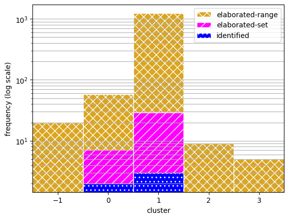
fig.savefig("outputs_paper_jmd_synthetic_modes/cluster_dist.pdf", format="pdf", bbox_inches = 'tight', pad_inches = 0)
fig.savefig("outputs_paper_jmd_synthetic_modes/cluster_dist.eps", format="eps", bbox_inches = 'tight', pad_inches = 0)
The PostScript backend does not support transparency; partially transparent artists will be rendered opaque.
Next, summarizing the overall stats from the approaches:
uncat_range = sum([i==-1 for i in cat_range])
uncat_set = sum([i==-1 for i in cat_set])
uncat_id = sum([i==-1 for i in cat_id])
uncat = [uncat_id, uncat_set, uncat_range]
lens = [len(X_id), len(X_set), len(X_range)]
num_cat = 100*np.array([len(set(cat_id))/len(unique_labels),len(set(cat_set))/len(unique_labels),len(set(cat_range))/len(unique_labels)])
res_tab = pd.DataFrame([lens, sim_times,num_cat, uncat])
res_tab.columns=['Identified', 'Elaborated-Set', 'Elaborated-Range']
res_tab.index=["Scenarios","Comp. Time (s)", "% Clusters", "Unclustered"]
res_tab
| Identified | Elaborated-Set | Elaborated-Range | |
|---|---|---|---|
| Scenarios | 5.000000 | 36.000000 | 1331.000000 |
| Comp. Time (s) | 4.779684 | 5.938389 | 90.814953 |
| % Clusters | 40.000000 | 40.000000 | 100.000000 |
| Unclustered | 0.000000 | 0.000000 | 20.000000 |
print(res_tab.to_latex(float_format="%.2f"))
\begin{tabular}{lrrr}
\toprule
 & Identified & Elaborated-Set & Elaborated-Range \\
\midrule
Scenarios & 5.00 & 36.00 & 1331.00 \\
Comp. Time (s) & 4.78 & 5.94 & 90.81 \\
% Clusters & 40.00 & 40.00 & 100.00 \\
Unclustered & 0.00 & 0.00 & 20.00 \\
\bottomrule
\end{tabular}
Finally, we use the following to calculate more detailed statistics about the cluster coverage.
def calc_2d_cov_loss(xmin, xmax, ymin, ymax, xs, ys):
    return calc_coverage_loss(xmin, xmax, xs)*calc_coverage_loss(ymin, ymax, ys)
def calc_coverage_loss(xmin, xmax, xs):
    if xs:
        return (xmax-np.max(xs)+np.min(xs)-xmin)/(xmax-xmin)
    else:
        return  (xmax-xmin)/(xmax-xmin)
def get_xs_ys(values, X_type):
    return [v[0] for v in values if v in X_type], [v[1] for v in values if v in X_type]
cov_loss_id,cov_loss_set,cov_loss_range = [],[],[]
num_scens_id,num_scens_set,num_scens_range = [],[],[]
for cat, values in cat_values.items():
    xs = [v[0] for v in values]
    ys = [v[1] for v in values]
    xs_id, ys_id = get_xs_ys(values, X_id)
    xs_set, ys_set = get_xs_ys(values, X_set)
    xs_range, ys_range = get_xs_ys(values, X_range)
    xmin,xmax,ymin,ymax = np.min(xs), np.max(xs), np.min(ys), np.max(ys)

    cov_loss_id.append(calc_2d_cov_loss(xmin,xmax,ymin,ymax ,xs_id,ys_id))
    cov_loss_set.append(calc_2d_cov_loss(xmin,xmax,ymin,ymax ,xs_set,ys_set))
    cov_loss_range.append(calc_2d_cov_loss(xmin,xmax,ymin,ymax, xs_range,ys_range))

    num_scens_id.append(len(xs_id));num_scens_set.append(len(xs_set));num_scens_range.append(len(xs_range))
Coverage Compared to the range approach:
cov_tab = pd.DataFrame([cov_loss_id,cov_loss_set,cov_loss_range], columns=list(cat_values.keys()), index = ["Identified", "Set", "Range"])

cov_tab
| 0 | 1 | 2 | 3 | -1 | |
|---|---|---|---|---|---|
| Identified | 0.704326 | 0.348938 | 1.0 | 1.0 | 1.0 |
| Set | 0.073416 | 0.116869 | 1.0 | 1.0 | 1.0 |
| Range | 0.000000 | 0.000000 | 0.0 | 0.0 | 0.0 |
Number of scenarios per approach for each cluster:
scens_tab = pd.DataFrame([num_scens_id,num_scens_set,num_scens_range], columns=list(cat_values.keys()), index = ["Identified", "Set", "Range"], dtype=int)

scens_tab
| 0 | 1 | 2 | 3 | -1 | |
|---|---|---|---|---|---|
| Identified | 2 | 3 | 0 | 0 | 0 |
| Set | 7 | 18 | 0 | 0 | 0 |
| Range | 39 | 933 | 5 | 4 | 10 |
len(cat_values[0])
45
Combined Table:
comb = pd.concat({"# Scenarios":scens_tab, "Coverage Loss":cov_tab, "Worst-Case":cat_tab}, axis="columns",join='inner')
comb = comb.swaplevel(0, axis="columns")
#index = pd.MultiIndex.from_tuples(comb.columns)
#comb = comb.reindex(index, axis="columns")
comb = comb.sort_index(axis="columns")
comb = comb.T
#comb_2.index = comb.index
comb
| Identified | Set | Range | ||
|---|---|---|---|---|
| -1 | # Scenarios | 0.000000 | 0.000000 | 10.000000 |
| Coverage Loss | 1.000000 | 1.000000 | 0.000000 | |
| Worst-Case | 0.000000 | 0.000000 | 11.962856 | |
| 0 | # Scenarios | 2.000000 | 7.000000 | 39.000000 |
| Coverage Loss | 0.704326 | 0.073416 | 0.000000 | |
| Worst-Case | 0.000000 | 0.556991 | 0.000000 | |
| 1 | # Scenarios | 3.000000 | 18.000000 | 933.000000 |
| Coverage Loss | 0.348938 | 0.116869 | 0.000000 | |
| Worst-Case | 18.536162 | 18.536162 | 18.621225 | |
| 2 | # Scenarios | 0.000000 | 0.000000 | 5.000000 |
| Coverage Loss | 1.000000 | 1.000000 | 0.000000 | |
| Worst-Case | 0.000000 | 0.000000 | 13.672471 | |
| 3 | # Scenarios | 0.000000 | 0.000000 | 4.000000 |
| Coverage Loss | 1.000000 | 1.000000 | 0.000000 | |
| Worst-Case | 0.000000 | 0.000000 | 1.619383 |
print(comb.to_latex( ))
\begin{tabular}{llrrr}
\toprule
 &  & Identified & Set & Range \\
\midrule
\multirow[t]{3}{*}{-1} & # Scenarios & 0.000000 & 0.000000 & 10.000000 \\
 & Coverage Loss & 1.000000 & 1.000000 & 0.000000 \\
 & Worst-Case & 0.000000 & 0.000000 & 11.962856 \\
\cline{1-5}
\multirow[t]{3}{*}{0} & # Scenarios & 2.000000 & 7.000000 & 39.000000 \\
 & Coverage Loss & 0.704326 & 0.073416 & 0.000000 \\
 & Worst-Case & 0.000000 & 0.556991 & 0.000000 \\
\cline{1-5}
\multirow[t]{3}{*}{1} & # Scenarios & 3.000000 & 18.000000 & 933.000000 \\
 & Coverage Loss & 0.348938 & 0.116869 & 0.000000 \\
 & Worst-Case & 18.536162 & 18.536162 & 18.621225 \\
\cline{1-5}
\multirow[t]{3}{*}{2} & # Scenarios & 0.000000 & 0.000000 & 5.000000 \\
 & Coverage Loss & 1.000000 & 1.000000 & 0.000000 \\
 & Worst-Case & 0.000000 & 0.000000 & 13.672471 \\
\cline{1-5}
\multirow[t]{3}{*}{3} & # Scenarios & 0.000000 & 0.000000 & 4.000000 \\
 & Coverage Loss & 1.000000 & 1.000000 & 0.000000 \\
 & Worst-Case & 0.000000 & 0.000000 & 1.619383 \\
\cline{1-5}
\bottomrule
\end{tabular}