Downloading and interpreting TEMPO Data Files programmatically from NASA Earthdata.

Published

September 8, 2025

Demonstration for working with TEMPO data via Harmony-py

Overview

This hands-on tutorial demonstrates how to programmatically access and analyze TEMPO air quality data using Python to monitor air quality impacts from the Madre wildfire. You’ll learn to efficiently download TEMPO NO₂ data using harmony-py, apply quality filtering, and create maps of air quality data showing wildfire emission patterns.

Why programmatic access? Automate data retrieval for regular monitoring workflows, batch processing, and reproducible analysis—building on the browser-based download methods you’ve already learned.

Tutorial Navigation: Variables and text highlighted in yellow are key parameters you’ll likely want to modify for your own region, time period, or data requirements.

Prerequisites

Required: - Free NASA Earthdata Login account - Basic Python knowledge (variables, loops, functions) - Familiarity with TEMPO instrument and data products (from previous presentations)

Python Libraries: - cartopy - for map projections and geographic visualization - harmony-py - for accessing NASA’s Harmony data services - matplotlib - for creating plots and visualizations - numpy - for numerical operations - xarray - for working with multi-dimensional scientific data

Data & Scope

Product: TEMPO_NO2_L3_V03 (Level-3 gridded NO₂ columns)
Resolution: approximately 2.1 km × 4.4 km, hourly during daylight
Coverage: North America
Example region: Madre wildfire area, New Cuyama, California

Methods apply to other TEMPO products (formaldehyde, ozone, etc.) and regions within North America.

Notebook Author / Affiliation

Author: Dr. Daniel Kaufman / Atmospheric Science Data Center
This notebook is based on examples from the harmony-py repository and Harmony documentation.

1. Setup

Install required packages (these may not be pre-installed in all environments)

!pip install --quiet harmony-py cartopy

Import Python libraries for data access, processing, and visualization

# For Section 2. Downloading TEMPO data
import datetime as dt
import getpass
import os
from harmony import BBox, Client, Collection, Request

# For Section 3. Opening TEMPO data files
import xarray as xr

# For Section 4. Creating graphics for a TEMPO data variable
import cartopy.crs as ccrs
import cartopy.feature as cfeature
import matplotlib.pyplot as plt
from cartopy.mpl.gridliner import LONGITUDE_FORMATTER, LATITUDE_FORMATTER
from xarray.plot.utils import label_from_attrs

2. Downloading TEMPO data (via Harmony)

Estimated time: 2-5 minutes for this example (it will depend on data size and network speed)

2.1 Authentication with NASA Earthdata

Enter your Earthdata Login credentials (username and password) to access TEMPO data. Your credentials are securely passed to NASA’s servers and are not stored in this notebook.

print("Please provide your Earthdata Login credentials to allow data access")
print("Your credentials will only be passed to Earthdata and will not be exposed in the notebook")

Please provide your Earthdata Login credentials to allow data access
Your credentials will only be passed to Earthdata and will not be exposed in the notebook

username = input("Username:")

harmony_client = Client(auth=(username, getpass.getpass()))

Username: dkaufas
 ········

2.2 Compiling a Request

Finding Collection IDs: Search for “TEMPO_NO2_L3” in NASA Earthdata Search, select your desired version, and copy the collection ID from the URL.

Building a Data Request: Configure your data request by specifying the data collection (i.e., NO₂, CH₂O, O₃; Processing Level; and Version, via Collection), time period (via temporal), and geographic area of interest (via spatial). The example below requests data for a 15-minute window over the central United States.

print(f"This tutorial will download data for: {dt.datetime(2025, 7, 3, 20, 0, 0)} UTC")
print("This corresponds to approximately 1:00 PM Pacific time during the Madre wildfire")

This tutorial will download data for: 2025-07-03 20:00:00 UTC
This corresponds to approximately 1:00 PM Pacific time during the Madre wildfire

print("Note: TEMPO times are in UTC. For western US:")
print("- PST = UTC - 8 hours")
print("- PDT = UTC - 7 hours")
print("- MST = UTC - 7 hours")
print("- MDT = UTC - 6 hours")

Note: TEMPO times are in UTC. For western US:
- PST = UTC - 8 hours
- PDT = UTC - 7 hours
- MST = UTC - 7 hours
- MDT = UTC - 6 hours

Spatial Coverage: The following example uses a rectangle that covers the Madre wildfire area near New Cuyama, California: - Longitude: -121° to -119° (2° wide) - Latitude: 34° to 36° (2° tall)

View the coverage area

request = Request(
    # This ID is for the Level-2, V03, "Nitrogen Dioxide total column" collection:
    # collection=Collection(id="C2930725014-LARC_CLOUD"),
    # This ID is for the Level-3, V03, "Nitrogen Dioxide tropospheric and stratospheric columns" collection:
    collection=Collection(id="C2930763263-LARC_CLOUD"),
    # This is a 15 minute time period (reminder, it's in UTC time):
    temporal={
        "start": dt.datetime(2025, 7, 3, 20, 0, 0),  # Day after fire start
        "stop": dt.datetime(2025, 7, 3, 20, 15, 0),
    },
    # This is a rectangular area in California
    spatial=BBox(-121, 34, -119, 36),  # New Cuyama area
    # Note that there is not a particular granule specified!
    # However, one could be specified by passing a granule ID, e.g.:
    #
    # granule_name=["TEMPO_NO2_L2_V03_20250406T215103Z_S012G07.nc"],
    #
)

# Validate the request before submitting
print("Request validation:")
print(f"✓ Valid request: {request.is_valid()}")
print(f"✓ Time period: {request.temporal['start']} to {request.temporal['stop']}")
print(f"✓ Spatial bounds: {request.spatial}")

Request validation:
✓ Valid request: True
✓ Time period: 2025-07-03 20:00:00 to 2025-07-03 20:15:00
✓ Spatial bounds: BBox: West:-121, South:34, East:-119, North:36

2.3 Submit and Monitor the Request

Submit your request to Harmony’s processing queue. The job ID allows you to track processing status.

job_id = harmony_client.submit(request)
print(f"jobID = {job_id}")

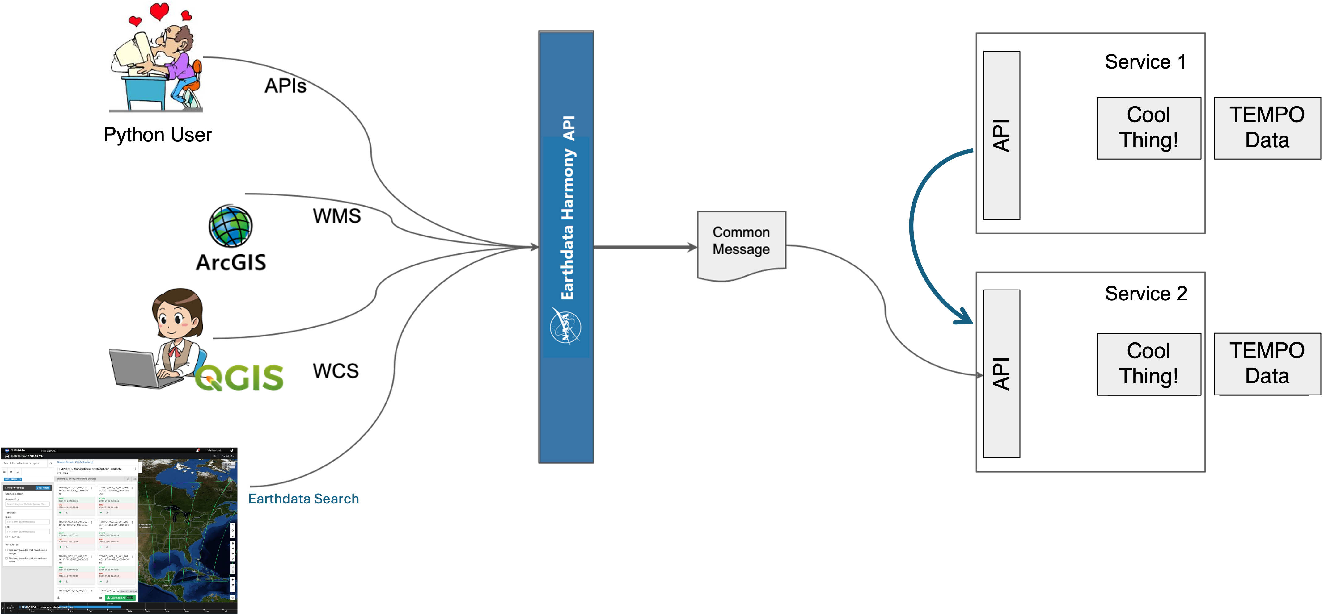
harmony_client.wait_for_processing(job_id, show_progress=True)

jobID = 808d5b8f-a3c5-4110-8ca0-0798bac99c4f

 [ Processing: 100% ] |###################################################| [|]

What is Harmony?

Harmony is the cloud services orchestrator for NASA Earth Science Data and Information System (ESDIS). The goal of Harmony is to provide services to increase usage and ease of use of ESDIS’ Earth observation data, especially focusing on opportunities made possible by cloud-accessible data.

Data processed by Harmony are staged in Amazon s3 buckets, and Harmony services run in containers in pods in a Kubernetes cluster.

Note that services provided via Harmony can transform NASA data as well as provide access to the original data, through an Application Programmable Interface (API). Harmony and its services can be invoked via wrapper libraries such as harmony-py as well as through curl commands, e.g.:

https://harmony.earthdata.nasa.gov/{collectionId}/ogc-api-coverages/1.0.0/{variable}/coverage/rangeset

(Harmony services REST API conforms to the OGC Coverages API version 1.0.0. It accepts parameters in the URL path as well as query parameters.)

2.4 Download Processed Data

Download the subset data files to your local system. Files are saved to a tempo_data folder (download_dir) in your home directory.

download_dir = os.path.expanduser("~/tempo_data")
os.makedirs(download_dir, exist_ok=True)

results = harmony_client.download_all(job_id, directory=download_dir)
all_results_stored = [f.result() for f in results]

/home/jovyan/tempo_data/106108034_TEMPO_NO2_L3_V03_20250703T190954Z_S011_subsetted.nc4
/home/jovyan/tempo_data/106108035_TEMPO_NO2_L3_V03_20250703T200954Z_S012_subsetted.nc4

print("✓ Data downloaded successfully!")
print(f"✓ Files saved to: {download_dir}")
print(f"✓ Number of files: {len(all_results_stored)}")

✓ Data downloaded successfully!
✓ Files saved to: /home/jovyan/tempo_data
✓ Number of files: 2

2.5 Troubleshooting Common Issues

Authentication errors: Verify your Earthdata Login credentials are correct

No data returned: - Check that your time period is after August 2023 (TEMPO operational start) - Verify your spatial bounds overlap with the TEMPO Field of Regard in North America - Try a broader time window (TEMPO has hourly coverage during daylight)

Large downloads: Start with smaller spatial areas or shorter time periods for testing

Memory issues: Close other applications or process files individually rather than loading multiple simultaneously

3. Opening TEMPO data files

Alternative Entry Point

If you already have TEMPO data files (downloaded via Earthdata Search or other methods), you can start here by pointing to your file location.

To use your own data: Replace the file_path below with your data file location:

file_path = all_results_stored[0]

print(f"file path: {file_path}")

file path: /home/jovyan/tempo_data/106108034_TEMPO_NO2_L3_V03_20250703T190954Z_S011_subsetted.nc4

In the following cell, we open the file, and can inspect the preview of data file groups, dimensions, time and space coordinates, data variables, and other attributes.

datatree = xr.open_datatree(file_path)
datatree

4. Creating graphics for a TEMPO data variable

Visualizing NO₂ Data

Let’s examine the tropospheric NO₂ column data (specified by vertical_column_troposphere, which is in the “product” group) - this represents the total amount of NO₂ in the lower atmosphere, which is most relevant for air quality applications.

data_array = datatree["product/vertical_column_troposphere"]
data_array

underlying_array = data_array.values
print(f"Type of underlying array: {type(underlying_array)}")

Type of underlying array: <class 'numpy.ndarray'>

4.1 Apply Quality Control

TEMPO provides quality flags to help identify reliable measurements: - 0 = Normal quality (use for analysis) - 1 = Suspect quality (use with caution) - 2 = Bad quality (exclude from analysis)

We’ll filter to show only high-quality data.

quality_flags = datatree["product/main_data_quality_flag"]
quality_flags

good_array = data_array.where(quality_flags == 0).squeeze()
good_array

print(f"Data size in memory: {good_array.nbytes / 1e6:.1f} MB")

Data size in memory: 0.1 MB

# Let's do a general look at the values.
print(
    f"Data range: {good_array.min().values:.2e} to {good_array.max().values:.2e} {data_array.attrs.get('units', '')}"
)
print(f"Mean value: {good_array.mean().values:.2e}")

Data range: -3.80e+15 to 3.49e+16 molecules/cm^2
Mean value: 1.61e+15

print("\nFor reference:")
print(
    "- Typical moderate to heavily polluted urban NO₂ tropospheric columns: >5×10¹⁵ molecules/cm²"
)
print("- Typical rural areas: <5×10¹⁵ molecules/cm²")
print("- Wildfire-affected areas: May show elevated NO₂ from combustion processes")


For reference:
- Typical moderate to heavily polluted urban NO₂ tropospheric columns: >5×10¹⁵ molecules/cm²
- Typical rural areas: <5×10¹⁵ molecules/cm²
- Wildfire-affected areas: May show elevated NO₂ from combustion processes

4.2 Create a Good-looking Map

Generate a publication-ready map showing NO₂ concentrations with major roads and coordinate labels, within a broader regional extent.

data_proj = ccrs.PlateCarree()

roads = cfeature.NaturalEarthFeature(
    category="cultural",
    name="roads",
    scale="10m",  # The dataset scale (e.g., '10m', '50m', '110m')
    facecolor="grey",
)

## If you wanted to add County boundaries, you could un-comment the following lines
##    and the axis.add_feature() call below
# admin_2_counties = cfeature.NaturalEarthFeature(
#     category='cultural',
#     name='admin_2_counties',
#     scale='10m',  # The dataset scale (e.g., '10m', '50m', '110m')
#     facecolor='none'
# )


def make_nice_map(axis):
    axis.set_extent([-122, -118, 33.5, 36.5], crs=data_proj)  # Central California

    axis.add_feature(cfeature.OCEAN, color="lightblue")
    axis.add_feature(cfeature.STATES, color="grey", linewidth=1)
    axis.add_feature(roads, linestyle="-", edgecolor="white", linewidth=0.8)
    # axis.add_feature(admin_2_counties, edgecolor='white', linewidth=0.3)

    grid = axis.gridlines(draw_labels=["left", "bottom"], dms=True, linestyle=":")
    grid.xformatter = LONGITUDE_FORMATTER
    grid.yformatter = LATITUDE_FORMATTER

fig, ax = plt.subplots(figsize=(10, 6), subplot_kw={"projection": data_proj})

make_nice_map(ax)

contour_handle = ax.contourf(
    datatree["geolocation/longitude"],
    datatree["geolocation/latitude"],
    good_array,
    levels=30,
    vmin=0,
    vmax=float(good_array.max()),
    alpha=0.6,
    cmap="inferno",
    zorder=2,
)

cb = plt.colorbar(contour_handle)
cb.set_label(label_from_attrs(data_array))

plt.show()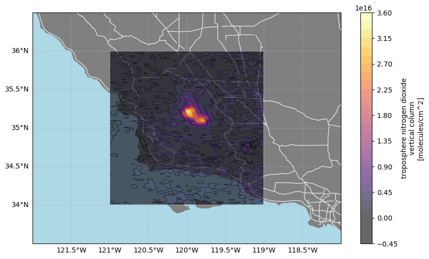

print("✓ Map created successfully!")
print("✓ Tutorial complete - you've successfully accessed and visualized TEMPO data!")

✓ Map created successfully!
✓ Tutorial complete - you've successfully accessed and visualized TEMPO data!

Tutorial Complete

What you accomplished: - ✅ Set up programmatic access to NASA TEMPO data - ✅ Downloaded and subset TEMPO NO₂ data for a specific region and time - ✅ Applied quality filtering to ensure reliable measurements
- ✅ Created a professional map visualization of air quality data

Key skills gained: - Using harmony-py for NASA data access - Working with TEMPO data structure and quality flags - Creating publication-ready maps with cartopy and matplotlib

You now have the foundation to adapt this workflow for your own air quality monitoring needs!

Potential Next Steps for Air Quality Analyses

This tutorial covered basic TEMPO data access via Harmony. Consider these extensions:

Analysis Expansions: - Time series analysis across multiple periods - Integration with ground monitoring stations

Alternative Access Methods: - earthaccess package - Simplified NASA data access - VirtualiZarr - Cloud-native analysis without downloads - Direct cloud access - AWS S3 integration for large-scale processing

Operational Applications: - Multi-pollutant analysis (NO₂ + formaldehyde + ozone) - Automated monitoring workflows - Cross-platform validation studies

While we won’t have time to cover most of these topics in detail, we may be able to incorporate some into Day 3 activities or discuss them further after the training sessions.