import earthaccess
import numpy as np
from matplotlib import pyplot as plt
from pyhdf.SD import SD, SDCCALIPSO Ozone Number Density
Summary
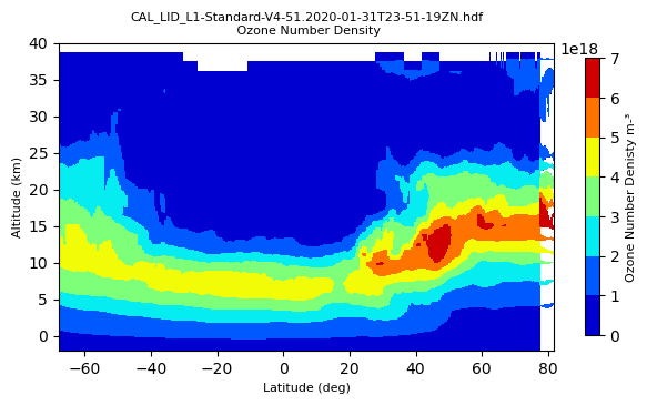
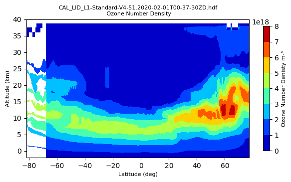
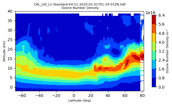
This notebook shows how to plot the vertical distribution of ozone number density (\(m^{-3}\)) from the Cloud-Aerosol Lidar and Infrared Pathfinder Satellite Observations (CALIPSO) using the pyhdf library for a latitudinal section. The particular data used here are CALIPSO Lidar Level 1B profile data, V4-51.
Prerequisites
A free(!) account at https://www.earthdata.nasa.gov/ is needed to login and download the appropriate files.
This notebook was last tested using Python 3.10.15, and requires these libraries:
1. Setup
2. Search for data using earthaccess
We use earthaccess to streamline the login to NASA Earthdata.
Additional resources about earthaccess
earthaccess.login()<earthaccess.auth.Auth at 0x118ed9f00>short_name = "CAL_LID_L1-Standard-V4-51"
version = "V4-51"
results = earthaccess.search_data(
short_name=short_name, version=version, temporal=("2020-02-01T00:00:00", "2020-02-01T01:59:59")
)
print(f"{len(results)} file(s) found.")3 file(s) found.print(results)[Collection: {'ShortName': 'CAL_LID_L1-Standard-V4-51', 'Version': 'V4-51'}
Spatial coverage: {'HorizontalSpatialDomain': {'Geometry': {'Lines': [{'Points': [{'Latitude': 77.436340332, 'Longitude': 171.039031982}, {'Latitude': 78.455823444, 'Longitude': 166.593692496}, {'Latitude': 79.336905179, 'Longitude': 161.706260626}, {'Latitude': 80.713705914, 'Longitude': 150.453975049}, {'Latitude': 81.592728206, 'Longitude': 137.033875562}, {'Latitude': 81.932023286, 'Longitude': 122.000871143}, {'Latitude': 81.697649597, 'Longitude': 106.710576372}, {'Latitude': 80.907042948, 'Longitude': 92.826795648}, {'Latitude': 79.607779782, 'Longitude': 81.123792826}, {'Latitude': 78.766029263, 'Longitude': 76.04493013}, {'Latitude': 76.551638952, 'Longitude': 66.481551943}, {'Latitude': 75.115071453, 'Longitude': 62.047476577}, {'Latitude': 73.470198105, 'Longitude': 58.098948508}, {'Latitude': 71.581951507, 'Longitude': 54.5517683}, {'Latitude': 69.436221619, 'Longitude': 51.381833235}, {'Latitude': 67.00220593, 'Longitude': 48.539908801}, {'Latitude': 64.239344907, 'Longitude': 45.979124835}, {'Latitude': 61.114295959, 'Longitude': 43.669269562}, {'Latitude': 57.404864049, 'Longitude': 41.186174644}, {'Latitude': 53.187384807, 'Longitude': 38.936621212}, {'Latitude': 48.383831835, 'Longitude': 36.877423613}, {'Latitude': 34.52514958, 'Longitude': 32.314445011}, {'Latitude': 24.364261627, 'Longitude': 29.746038437}, {'Latitude': -23.170105881, 'Longitude': 19.269805017}, {'Latitude': -31.546138763, 'Longitude': 17.111696243}, {'Latitude': -41.699597557, 'Longitude': 14.208567538}, {'Latitude': -46.029007304, 'Longitude': 12.67270214}, {'Latitude': -55.533259073, 'Longitude': 8.557231096}, {'Latitude': -60.29538009, 'Longitude': 5.763747606}, {'Latitude': -64.358884268, 'Longitude': 2.596728101}, {'Latitude': -67.816558838, 'Longitude': -1.016557336}]}]}}}
Temporal coverage: {'RangeDateTime': {'BeginningDateTime': '2020-01-31T23:51:17.288+00:00', 'EndingDateTime': '2020-02-01T00:37:28.589+00:00'}}
Size(MB): 0
Data: ['https://asdc.larc.nasa.gov/data/CALIPSO/LID_L1-Standard-V4-51/2020/01/CAL_LID_L1-Standard-V4-51.2020-01-31T23-51-19ZN.hdf'], Collection: {'ShortName': 'CAL_LID_L1-Standard-V4-51', 'Version': 'V4-51'}
Spatial coverage: {'HorizontalSpatialDomain': {'Geometry': {'Lines': [{'Points': [{'Latitude': -67.824928284, 'Longitude': -1.026128411}, {'Latitude': -69.720491457, 'Longitude': -3.26099699}, {'Latitude': -71.437554837, 'Longitude': -5.703259778}, {'Latitude': -72.983768051, 'Longitude': -8.363793397}, {'Latitude': -74.374526544, 'Longitude': -11.266338106}, {'Latitude': -75.624426511, 'Longitude': -14.440531322}, {'Latitude': -76.746920136, 'Longitude': -17.924412141}, {'Latitude': -78.629885585, 'Longitude': -25.902122221}, {'Latitude': -80.099286824, 'Longitude': -35.652219973}, {'Latitude': -81.131191352, 'Longitude': -47.179296989}, {'Latitude': -81.717446691, 'Longitude': -60.44870905}, {'Latitude': -81.818862915, 'Longitude': -74.655960083}, {'Latitude': -81.543302144, 'Longitude': -88.161353156}, {'Latitude': -80.821570755, 'Longitude': -100.519894639}, {'Latitude': -79.688794105, 'Longitude': -111.146471596}, {'Latitude': -78.139527358, 'Longitude': -120.144710133}, {'Latitude': -76.186541051, 'Longitude': -127.558075791}, {'Latitude': -75.027234568, 'Longitude': -130.821198761}, {'Latitude': -73.743230284, 'Longitude': -133.797961466}, {'Latitude': -72.320680604, 'Longitude': -136.525195792}, {'Latitude': -70.744670644, 'Longitude': -139.031146968}, {'Latitude': -69.007762661, 'Longitude': -141.328133863}, {'Latitude': -65.240990464, 'Longitude': -145.404140833}, {'Latitude': -63.222711374, 'Longitude': -147.231335217}, {'Latitude': -61.022577926, 'Longitude': -148.935128749}, {'Latitude': -58.632229758, 'Longitude': -150.523042124}, {'Latitude': -53.195430685, 'Longitude': -153.409405747}, {'Latitude': -42.342311669, 'Longitude': -157.627441906}, {'Latitude': -37.449474233, 'Longitude': -159.198822075}, {'Latitude': -25.827674866, 'Longitude': -162.228530884}, {'Latitude': -16.684080293, 'Longitude': -164.417013885}, {'Latitude': 16.445716858, 'Longitude': -171.551559448}, {'Latitude': 28.119762899, 'Longitude': -174.254328626}, {'Latitude': 42.603369779, 'Longitude': -178.41590732}, {'Latitude': 47.155918741, 'Longitude': -180}]}, {'Points': [{'Latitude': 47.155918741, 'Longitude': 180}, {'Latitude': 53.162760112, 'Longitude': 177.416908617}, {'Latitude': 58.284416199, 'Longitude': 174.533126831}, {'Latitude': 61.949400119, 'Longitude': 172.239661965}, {'Latitude': 65.1701292, 'Longitude': 169.684072191}, {'Latitude': 67.988793651, 'Longitude': 166.8312067}, {'Latitude': 70.446788893, 'Longitude': 163.642454722}, {'Latitude': 72.592132022, 'Longitude': 160.057661741}, {'Latitude': 74.462272838, 'Longitude': 156.008101364}, {'Latitude': 76.077069907, 'Longitude': 151.444997414}, {'Latitude': 77.454971313, 'Longitude': 146.323318481}]}]}}}
Temporal coverage: {'RangeDateTime': {'BeginningDateTime': '2020-02-01T00:37:28.639+00:00', 'EndingDateTime': '2020-02-01T01:29:49.666+00:00'}}
Size(MB): 0
Data: ['https://asdc.larc.nasa.gov/data/CALIPSO/LID_L1-Standard-V4-51/2020/02/CAL_LID_L1-Standard-V4-51.2020-02-01T00-37-30ZD.hdf'], Collection: {'ShortName': 'CAL_LID_L1-Standard-V4-51', 'Version': 'V4-51'}
Spatial coverage: {'HorizontalSpatialDomain': {'Geometry': {'Lines': [{'Points': [{'Latitude': 77.468635559, 'Longitude': 146.26763916}, {'Latitude': 78.479625249, 'Longitude': 141.829620195}, {'Latitude': 79.358659957, 'Longitude': 136.920804562}, {'Latitude': 80.730021529, 'Longitude': 125.622113233}, {'Latitude': 81.601559554, 'Longitude': 112.159736207}, {'Latitude': 81.931733658, 'Longitude': 97.106575105}, {'Latitude': 81.687931666, 'Longitude': 81.830304475}, {'Latitude': 80.88917308, 'Longitude': 67.986210985}, {'Latitude': 79.583662093, 'Longitude': 56.329840111}, {'Latitude': 78.739430334, 'Longitude': 51.272950637}, {'Latitude': 76.521301461, 'Longitude': 41.752012601}, {'Latitude': 75.083584015, 'Longitude': 37.336887847}, {'Latitude': 73.437959364, 'Longitude': 33.403976042}, {'Latitude': 71.549292128, 'Longitude': 29.869562817}, {'Latitude': 69.403426594, 'Longitude': 26.709864486}, {'Latitude': 66.96952087, 'Longitude': 23.876074022}, {'Latitude': 64.206988076, 'Longitude': 21.321710361}, {'Latitude': 61.082466125, 'Longitude': 19.016868591}, {'Latitude': 57.373823674, 'Longitude': 16.538239466}, {'Latitude': 53.157362494, 'Longitude': 14.292042012}, {'Latitude': 48.355057783, 'Longitude': 12.235336178}, {'Latitude': 34.500858075, 'Longitude': 7.676332119}, {'Latitude': 24.343690872, 'Longitude': 5.10929203}, {'Latitude': -23.18059551, 'Longitude': -5.36509496}, {'Latitude': -31.549236298, 'Longitude': -7.521789551}, {'Latitude': -41.696289695, 'Longitude': -10.423138022}, {'Latitude': -46.02672327, 'Longitude': -11.959264894}, {'Latitude': -55.524334823, 'Longitude': -16.07114686}, {'Latitude': -60.287460062, 'Longitude': -18.863983898}, {'Latitude': -64.351853617, 'Longitude': -22.030179149}, {'Latitude': -67.810325623, 'Longitude': -25.642435074}]}]}}}
Temporal coverage: {'RangeDateTime': {'BeginningDateTime': '2020-02-01T01:29:49.716+00:00', 'EndingDateTime': '2020-02-01T02:16:00.273+00:00'}}
Size(MB): 0
Data: ['https://asdc.larc.nasa.gov/data/CALIPSO/LID_L1-Standard-V4-51/2020/02/CAL_LID_L1-Standard-V4-51.2020-02-01T01-29-55ZN.hdf']]3. Download data
Note: The following download process will likely take a while, because each file is greater than 400 MB.
downloaded_files = earthaccess.download(results, local_path=".")
downloaded_files
['CAL_LID_L1-Standard-V4-51.2020-01-31T23-51-19ZN.hdf',
'CAL_LID_L1-Standard-V4-51.2020-02-01T00-37-30ZD.hdf',
'CAL_LID_L1-Standard-V4-51.2020-02-01T01-29-55ZN.hdf']4. Generate Plot
Ozone_number_density [# of single shot (333m) resn profiles in file (55725), met_data_altitude (33)]
for file in downloaded_files:
    # Retrieve data
    hdf = SD(file, SDC.READ)
    lat = hdf.select("Latitude").get()[:, 0]
    data = hdf.select("Ozone_Number_Density").get()
    ozone_number_density = np.transpose(data)

    # Interval for altitude to plot the y-axis.
    # Range is from -2 km - 40 km of 33 range bins. For more detail go to CALIPSO Data Products Catalog at:
    #   https://www-calipso.larc.nasa.gov/products/CALIPSO_DPC_Rev4x93.pdf
    met_data_altitudes = np.linspace(-2, 40, 33)

    # Plot data
    plt.figure(figsize=(7.20, 3.60))
    im = plt.contourf(lat, met_data_altitudes, ozone_number_density, cmap="jet")

    plt.title(f"{file}\n Ozone Number Density", fontsize=8)
    plt.ylabel("Altitude (km)", fontsize=8)
    plt.xlabel("Latitude (deg)", fontsize=8)

    cb = plt.colorbar(im, shrink=0.90)
    cb.set_label("Ozone Number Denisty m-³", fontsize=8)

    plt.savefig(f"{file}_Ozone_Number_Density.jpg", dpi=200)
    print(f"Plot has been saved: {file}_Ozone_Number_Density.jpg")
Plot has been saved: CAL_LID_L1-Standard-V4-51.2020-01-31T23-51-19ZN.hdf_Ozone_Number_Density.jpg
Plot has been saved: CAL_LID_L1-Standard-V4-51.2020-02-01T00-37-30ZD.hdf_Ozone_Number_Density.jpg
Plot has been saved: CAL_LID_L1-Standard-V4-51.2020-02-01T01-29-55ZN.hdf_Ozone_Number_Density.jpg