import cartopy.crs as ccrs
import earthaccess
import h5py
import matplotlib.pyplot as plt
import numpy as np
from cartopy.mpl.gridliner import LATITUDE_FORMATTER, LONGITUDE_FORMATTERPlotting DISCOVR EPIC Level-2 ozone product parameters
Summary
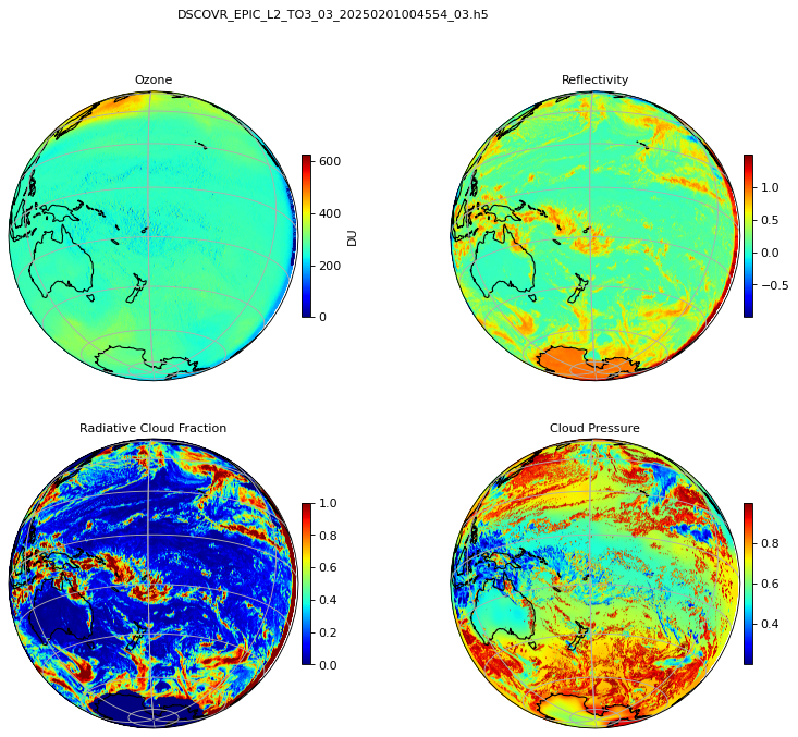
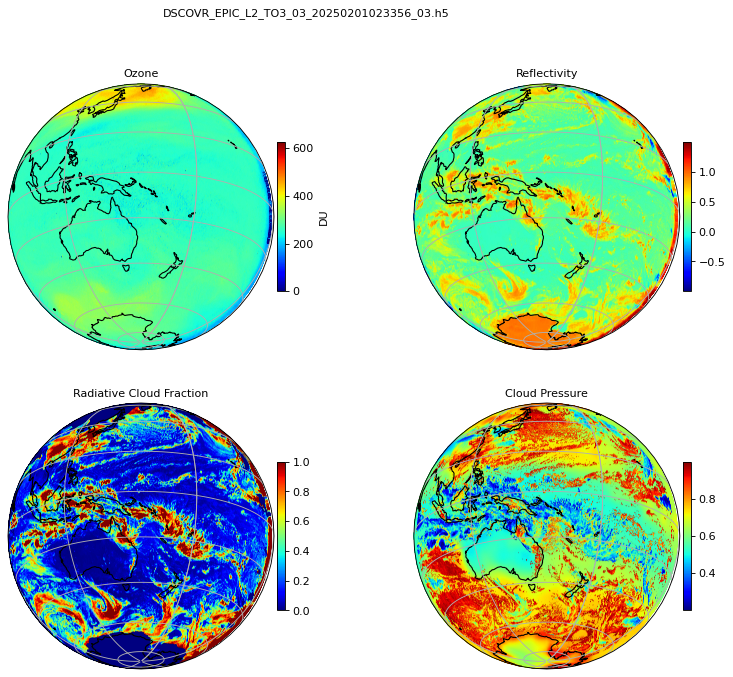
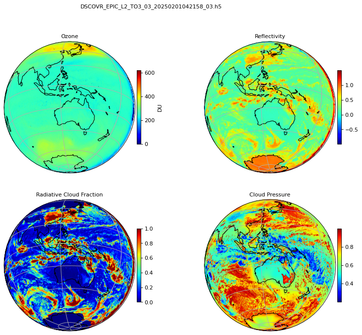
This code graphs 4 different parameters from the DSCOVR EPIC Level 2 Total Ozone, Version 3 product (Ozone, Reflectivity, Radiative Cloud Fraction, Cloud Pressure).
Reference
Code Reference: https://hdfeos.org/zoo/LaRC/DSCOVR_EPIC_L2_TO3_03_20210301005516_03.h5.py
For more information on this data product please vist: https://avdc.gsfc.nasa.gov/pub/DSCOVR/EPIC_Pulications/EPICTO3UserGuide_final.pdf
Prerequisites
A free(!) account at https://www.earthdata.nasa.gov/ is needed to login and download the appropriate files.
This notebook was written using Python 3.8.10, and requires these libraries:
1. Setup
2. Search for data using earthaccess
We use earthaccess to streamline the login to NASA Earthdata.
Additional resources about earthaccess
earthaccess.login()short_name = "DSCOVR_EPIC_L2_TO3"
version = "03"
results = earthaccess.search_data(
short_name=short_name,
version=version,
temporal=("2025-02-01T00:00:00", "2025-02-01T04:59:59"),
)
print(f"{len(results)} file(s) found.")3 file(s) found.print(results)[Collection: {'ShortName': 'DSCOVR_EPIC_L2_TO3', 'Version': '03'}
Spatial coverage: {'HorizontalSpatialDomain': {'Geometry': {'GPolygons': [{'Boundary': {'Points': [{'Latitude': 61.662150027, 'Longitude': 180}, {'Latitude': 60.881559768, 'Longitude': 170.550246061}, {'Latitude': 59.446416148, 'Longitude': 161.575307495}, {'Latitude': 57.385378569, 'Longitude': 153.243755735}, {'Latitude': 56.122062602, 'Longitude': 149.324365749}, {'Latitude': 54.706096953, 'Longitude': 145.575778651}, {'Latitude': 53.148679682, 'Longitude': 142.018043035}, {'Latitude': 51.433576429, 'Longitude': 138.607151533}, {'Latitude': 49.558332996, 'Longitude': 135.337891006}, {'Latitude': 47.513590642, 'Longitude': 132.194088825}, {'Latitude': 45.295254258, 'Longitude': 129.169700771}, {'Latitude': 42.898989395, 'Longitude': 126.257268024}, {'Latitude': 40.30613302, 'Longitude': 123.43351568}, {'Latitude': 37.503747539, 'Longitude': 120.685219083}, {'Latitude': 30.389841383, 'Longitude': 116.161716326}, {'Latitude': 21.961042992, 'Longitude': 111.674502076}, {'Latitude': 12.129531956, 'Longitude': 107.126244143}, {'Latitude': -2.953174538, 'Longitude': 100.739987202}, {'Latitude': -17.920211996, 'Longitude': 96.454447214}, {'Latitude': -28.801211566, 'Longitude': 92.862050392}, {'Latitude': -37.854263604, 'Longitude': 89.216515558}, {'Latitude': -41.789405152, 'Longitude': 87.328171092}, {'Latitude': -45.387280172, 'Longitude': 85.3697729}, {'Latitude': -50.499731789, 'Longitude': 83.258118692}, {'Latitude': -54.988782405, 'Longitude': 80.967249072}, {'Latitude': -58.932657459, 'Longitude': 78.457095563}, {'Latitude': -62.399565026, 'Longitude': 75.683232864}, {'Latitude': -65.439433938, 'Longitude': 72.604800134}, {'Latitude': -68.100676081, 'Longitude': 69.172613598}, {'Latitude': -70.421768371, 'Longitude': 65.337061221}, {'Latitude': -72.438914695, 'Longitude': 61.037826935}, {'Latitude': -74.218668983, 'Longitude': 56.090172697}, {'Latitude': -75.736403376, 'Longitude': 50.506776663}, {'Latitude': -77.002645232, 'Longitude': 44.243321011}, {'Latitude': -78.029411206, 'Longitude': 37.245454295}, {'Latitude': -78.831882039, 'Longitude': 29.353636303}, {'Latitude': -79.385848957, 'Longitude': 20.731332667}, {'Latitude': -79.681333176, 'Longitude': 11.500046226}, {'Latitude': -79.704868812, 'Longitude': 2.084472656}, {'Latitude': -79.681333176, 'Longitude': -7.331100913}, {'Latitude': -79.385848957, 'Longitude': -16.562387355}, {'Latitude': -78.831882039, 'Longitude': -25.184690991}, {'Latitude': -78.029411206, 'Longitude': -33.076508982}, {'Latitude': -77.002645232, 'Longitude': -40.074375698}, {'Latitude': -75.736403376, 'Longitude': -46.33783135}, {'Latitude': -74.218668983, 'Longitude': -51.921227384}, {'Latitude': -72.438914695, 'Longitude': -56.868881623}, {'Latitude': -70.421768371, 'Longitude': -61.168115908}, {'Latitude': -68.100676081, 'Longitude': -65.003668286}, {'Latitude': -65.439433938, 'Longitude': -68.435854821}, {'Latitude': -62.399565026, 'Longitude': -71.514287552}, {'Latitude': -58.932657459, 'Longitude': -74.288150251}, {'Latitude': -54.988782405, 'Longitude': -76.798303759}, {'Latitude': -50.499731789, 'Longitude': -79.089173379}, {'Latitude': -45.387280172, 'Longitude': -81.200827587}, {'Latitude': -41.789405152, 'Longitude': -83.159225779}, {'Latitude': -37.854263604, 'Longitude': -85.047570245}, {'Latitude': -28.801211566, 'Longitude': -88.693105079}, {'Latitude': -17.920211996, 'Longitude': -92.285501902}, {'Latitude': -2.953174538, 'Longitude': -96.57104189}, {'Latitude': 12.129531956, 'Longitude': -102.95729883}, {'Latitude': 21.961042992, 'Longitude': -107.505556764}, {'Latitude': 30.389841383, 'Longitude': -111.992771014}, {'Latitude': 37.503747539, 'Longitude': -116.516273771}, {'Latitude': 40.376546171, 'Longitude': -119.337393666}, {'Latitude': 43.029116414, 'Longitude': -122.238374121}, {'Latitude': 45.480978372, 'Longitude': -125.240775264}, {'Latitude': 47.737247324, 'Longitude': -128.350796854}, {'Latitude': 49.815327587, 'Longitude': -131.592918157}, {'Latitude': 51.712797785, 'Longitude': -134.963089885}, {'Latitude': 53.444692586, 'Longitude': -138.487494393}, {'Latitude': 55.012738167, 'Longitude': -142.171498621}, {'Latitude': 56.436780568, 'Longitude': -146.073231186}, {'Latitude': 57.695142616, 'Longitude': -150.144552517}, {'Latitude': 59.719552543, 'Longitude': -158.805853256}, {'Latitude': 61.080156756, 'Longitude': -168.138745384}, {'Latitude': 61.742680839, 'Longitude': -177.915527344}, {'Latitude': 61.662150027, 'Longitude': -180}, {'Latitude': -90, 'Longitude': -180}, {'Latitude': -90, 'Longitude': 180}, {'Latitude': 61.662150027, 'Longitude': 180}]}}]}}}
Temporal coverage: {'RangeDateTime': {'BeginningDateTime': '2025-02-01T00:41:06+00:00', 'EndingDateTime': '2025-02-01T00:47:41+00:00'}}
Size(MB): 198.10176849365234
Data: ['https://asdc.larc.nasa.gov/data/DSCOVR/EPIC/L2_TO3_03/2025/02/DSCOVR_EPIC_L2_TO3_03_20250201004554_03.h5'], Collection: {'ShortName': 'DSCOVR_EPIC_L2_TO3', 'Version': '03'}
Spatial coverage: {'HorizontalSpatialDomain': {'Geometry': {'GPolygons': [{'Boundary': {'Points': [{'Latitude': 58.511851145, 'Longitude': 180}, {'Latitude': 59.784395372, 'Longitude': 174.146906889}, {'Latitude': 60.760861627, 'Longitude': 168.007872498}, {'Latitude': 61.43315507, 'Longitude': 161.636947993}, {'Latitude': 61.795062873, 'Longitude': 155.089599609}, {'Latitude': 61.13176767, 'Longitude': 145.29669673}, {'Latitude': 59.772165979, 'Longitude': 135.967195473}, {'Latitude': 57.745661577, 'Longitude': 127.29483416}, {'Latitude': 56.485913495, 'Longitude': 123.219490416}, {'Latitude': 55.060310391, 'Longitude': 119.314718628}, {'Latitude': 53.490589031, 'Longitude': 115.628629127}, {'Latitude': 51.756913726, 'Longitude': 112.102975259}, {'Latitude': 49.857584963, 'Longitude': 108.732308464}, {'Latitude': 47.777578771, 'Longitude': 105.490362863}, {'Latitude': 45.519340779, 'Longitude': 102.381108479}, {'Latitude': 43.065470197, 'Longitude': 99.379995509}, {'Latitude': 40.403800964, 'Longitude': 96.47345426}, {'Latitude': 37.528763425, 'Longitude': 93.655047603}, {'Latitude': 30.411148768, 'Longitude': 89.138809636}, {'Latitude': 21.978532779, 'Longitude': 84.65975045}, {'Latitude': 12.143031118, 'Longitude': 80.120517632}, {'Latitude': -2.945436448, 'Longitude': 73.747786848}, {'Latitude': -17.916363439, 'Longitude': 69.476428464}, {'Latitude': -28.800640176, 'Longitude': 65.895907747}, {'Latitude': -37.857016085, 'Longitude': 62.262211328}, {'Latitude': -41.793874455, 'Longitude': 60.379851941}, {'Latitude': -45.393524215, 'Longitude': 58.427518604}, {'Latitude': -50.516494137, 'Longitude': 56.321952184}, {'Latitude': -55.016031761, 'Longitude': 54.03589284}, {'Latitude': -58.970324204, 'Longitude': 51.528566832}, {'Latitude': -62.439231532, 'Longitude': 48.761981887}, {'Latitude': -65.481218523, 'Longitude': 45.690073812}, {'Latitude': -68.144686978, 'Longitude': 42.263147433}, {'Latitude': -70.468086832, 'Longitude': 38.430871051}, {'Latitude': -72.487578792, 'Longitude': 34.131973863}, {'Latitude': -74.269698573, 'Longitude': 29.180336697}, {'Latitude': -75.789649869, 'Longitude': 23.5869741}, {'Latitude': -77.052313412, 'Longitude': 17.337543345}, {'Latitude': -78.081298351, 'Longitude': 10.318525991}, {'Latitude': -78.885343772, 'Longitude': 2.395052717}, {'Latitude': -79.437624748, 'Longitude': -6.221264488}, {'Latitude': -79.732904084, 'Longitude': -15.447655932}, {'Latitude': -79.757149372, 'Longitude': -24.910400391}, {'Latitude': -79.732904084, 'Longitude': -34.373144849}, {'Latitude': -79.437624748, 'Longitude': -43.599536293}, {'Latitude': -78.885343772, 'Longitude': -52.215853498}, {'Latitude': -78.081298351, 'Longitude': -60.139326772}, {'Latitude': -77.052313412, 'Longitude': -67.158344126}, {'Latitude': -75.789649869, 'Longitude': -73.407774881}, {'Latitude': -74.269698573, 'Longitude': -79.001137478}, {'Latitude': -72.487578792, 'Longitude': -83.952774644}, {'Latitude': -70.468086832, 'Longitude': -88.251671833}, {'Latitude': -68.144686978, 'Longitude': -92.083948214}, {'Latitude': -65.481218523, 'Longitude': -95.510874593}, {'Latitude': -62.439231532, 'Longitude': -98.582782668}, {'Latitude': -58.970324204, 'Longitude': -101.349367614}, {'Latitude': -55.016031761, 'Longitude': -103.856693621}, {'Latitude': -50.516494137, 'Longitude': -106.142752965}, {'Latitude': -45.393524215, 'Longitude': -108.248319386}, {'Latitude': -41.793874455, 'Longitude': -110.200652722}, {'Latitude': -37.857016085, 'Longitude': -112.08301211}, {'Latitude': -28.800640176, 'Longitude': -115.716708528}, {'Latitude': -17.916363439, 'Longitude': -119.297229245}, {'Latitude': -2.945436448, 'Longitude': -123.568587629}, {'Latitude': 12.143031118, 'Longitude': -129.941318413}, {'Latitude': 21.978532779, 'Longitude': -134.480551232}, {'Latitude': 30.411148768, 'Longitude': -138.959610417}, {'Latitude': 37.528763425, 'Longitude': -143.475848384}, {'Latitude': 41.324082738, 'Longitude': -147.263265393}, {'Latitude': 44.742405657, 'Longitude': -151.213534262}, {'Latitude': 47.80742642, 'Longitude': -155.354891625}, {'Latitude': 50.547054635, 'Longitude': -159.72562157}, {'Latitude': 52.979272541, 'Longitude': -164.35732629}, {'Latitude': 55.113094286, 'Longitude': -169.269511523}, {'Latitude': 56.954881012, 'Longitude': -174.47636564}, {'Latitude': 58.511851145, 'Longitude': -180}, {'Latitude': -90, 'Longitude': -180}, {'Latitude': -90, 'Longitude': 180}, {'Latitude': 58.511851145, 'Longitude': 180}]}}]}}}
Temporal coverage: {'RangeDateTime': {'BeginningDateTime': '2025-02-01T02:29:08+00:00', 'EndingDateTime': '2025-02-01T02:35:43+00:00'}}
Size(MB): 198.45312690734863
Data: ['https://asdc.larc.nasa.gov/data/DSCOVR/EPIC/L2_TO3_03/2025/02/DSCOVR_EPIC_L2_TO3_03_20250201023356_03.h5'], Collection: {'ShortName': 'DSCOVR_EPIC_L2_TO3', 'Version': '03'}
Spatial coverage: {'HorizontalSpatialDomain': {'Geometry': {'GPolygons': [{'Boundary': {'Points': [{'Latitude': 46.208063404, 'Longitude': 180}, {'Latitude': 49.655405829, 'Longitude': 174.909194022}, {'Latitude': 52.646422028, 'Longitude': 169.479169841}, {'Latitude': 55.215720437, 'Longitude': 163.646550274}, {'Latitude': 57.368350211, 'Longitude': 157.399126661}, {'Latitude': 59.127748827, 'Longitude': 150.650606521}, {'Latitude': 60.46658984, 'Longitude': 143.483974304}, {'Latitude': 61.378898122, 'Longitude': 135.930765807}, {'Latitude': 61.848171714, 'Longitude': 128.113037109}, {'Latitude': 61.184092114, 'Longitude': 118.303727478}, {'Latitude': 59.822323882, 'Longitude': 108.960743446}, {'Latitude': 58.891580616, 'Longitude': 104.54024117}, {'Latitude': 57.792614226, 'Longitude': 100.279000574}, {'Latitude': 56.53098397, 'Longitude': 96.200561613}, {'Latitude': 55.108460681, 'Longitude': 92.306592908}, {'Latitude': 53.537032513, 'Longitude': 88.6184027}, {'Latitude': 51.8015451, 'Longitude': 85.091498068}, {'Latitude': 49.900326025, 'Longitude': 81.720346681}, {'Latitude': 47.818362145, 'Longitude': 78.478597222}, {'Latitude': 45.551470809, 'Longitude': 75.361522767}, {'Latitude': 43.095340565, 'Longitude': 72.362423227}, {'Latitude': 40.431403451, 'Longitude': 69.458299294}, {'Latitude': 37.554097281, 'Longitude': 66.642651987}, {'Latitude': 30.440792925, 'Longitude': 62.138448706}, {'Latitude': 21.996247574, 'Longitude': 57.663013025}, {'Latitude': 12.156707636, 'Longitude': 53.13293768}, {'Latitude': -2.937588652, 'Longitude': 46.773926907}, {'Latitude': -17.921121208, 'Longitude': 42.514324862}, {'Latitude': -28.800034096, 'Longitude': 38.948473547}, {'Latitude': -37.859769005, 'Longitude': 35.326786363}, {'Latitude': -41.798362548, 'Longitude': 33.450500242}, {'Latitude': -45.399806215, 'Longitude': 31.504322799}, {'Latitude': -50.533318639, 'Longitude': 29.405031334}, {'Latitude': -55.043371931, 'Longitude': 27.123991259}, {'Latitude': -58.999685574, 'Longitude': 24.625690788}, {'Latitude': -62.479053506, 'Longitude': 21.860629203}, {'Latitude': -65.531304568, 'Longitude': 18.78625797}, {'Latitude': -68.196814916, 'Longitude': 15.362588529}, {'Latitude': -70.522284796, 'Longitude': 11.531070921}, {'Latitude': -72.53657298, 'Longitude': 7.246945024}, {'Latitude': -74.321118796, 'Longitude': 2.291497963}, {'Latitude': -75.837152923, 'Longitude': -3.285349935}, {'Latitude': -77.107965585, 'Longitude': -9.578812569}, {'Latitude': -78.13376146, 'Longitude': -16.587479783}, {'Latitude': -78.93593614, 'Longitude': -24.500223521}, {'Latitude': -79.490082083, 'Longitude': -33.153868075}, {'Latitude': -79.786042178, 'Longitude': -42.426152221}, {'Latitude': -79.810155569, 'Longitude': -51.886962891}, {'Latitude': -79.786042178, 'Longitude': -61.34777356}, {'Latitude': -79.490082083, 'Longitude': -70.620057706}, {'Latitude': -78.93593614, 'Longitude': -79.273702261}, {'Latitude': -78.13376146, 'Longitude': -87.186445998}, {'Latitude': -77.107965585, 'Longitude': -94.195113212}, {'Latitude': -75.837152923, 'Longitude': -100.488575846}, {'Latitude': -74.321118796, 'Longitude': -106.065423745}, {'Latitude': -72.53657298, 'Longitude': -111.020870806}, {'Latitude': -70.522284796, 'Longitude': -115.304996702}, {'Latitude': -68.196814916, 'Longitude': -119.13651431}, {'Latitude': -65.531304568, 'Longitude': -122.560183752}, {'Latitude': -62.479053506, 'Longitude': -125.634554984}, {'Latitude': -58.999685574, 'Longitude': -128.39961657}, {'Latitude': -55.043371931, 'Longitude': -130.89791704}, {'Latitude': -50.533318639, 'Longitude': -133.178957116}, {'Latitude': -45.399806215, 'Longitude': -135.27824858}, {'Latitude': -41.798362548, 'Longitude': -137.224426023}, {'Latitude': -37.859769005, 'Longitude': -139.100712144}, {'Latitude': -28.800034096, 'Longitude': -142.722399328}, {'Latitude': -17.921121208, 'Longitude': -146.288250644}, {'Latitude': -2.937588652, 'Longitude': -150.547852689}, {'Latitude': 12.156707636, 'Longitude': -156.906863461}, {'Latitude': 21.996247574, 'Longitude': -161.436938807}, {'Latitude': 30.440792925, 'Longitude': -165.912374487}, {'Latitude': 37.554097281, 'Longitude': -170.416577769}, {'Latitude': 42.166477527, 'Longitude': -175.086772884}, {'Latitude': 46.208063404, 'Longitude': -180}, {'Latitude': -90, 'Longitude': -180}, {'Latitude': -90, 'Longitude': 180}, {'Latitude': 46.208063404, 'Longitude': 180}]}}]}}}
Temporal coverage: {'RangeDateTime': {'BeginningDateTime': '2025-02-01T04:17:10+00:00', 'EndingDateTime': '2025-02-01T04:23:45+00:00'}}
Size(MB): 198.7623529434204
Data: ['https://asdc.larc.nasa.gov/data/DSCOVR/EPIC/L2_TO3_03/2025/02/DSCOVR_EPIC_L2_TO3_03_20250201042158_03.h5']]3. Download data
downloaded_files = earthaccess.download(results, local_path=".")
downloaded_files
['DSCOVR_EPIC_L2_TO3_03_20250201004554_03.h5',
'DSCOVR_EPIC_L2_TO3_03_20250201023356_03.h5',
'DSCOVR_EPIC_L2_TO3_03_20250201042158_03.h5']4. Open the files
arrays = {
    "ozone": [],
    "reflectivity": [],
    "rcf": [],
    "cp": [],
    "lon": [],
    "lat": [],
    "lon_m": [],
    "lat_m": [],
}

for file in downloaded_files:
    with h5py.File(file, mode="r") as f:
        ozone = f["/Ozone"][:].astype(np.float64)
        reflectivity = f["/Reflectivity"][:].astype(np.float64)
        RCF = f["/RadiativeCloudFraction"][:].astype(np.float64)
        CP = f["/CloudPressure"][:].astype(np.float64)
        lon = f["/Longitude"][:]
        lat = f["/Latitude"][:]

        # Set fill value for each variable
        FillValue = -999.0

        ozone[ozone == FillValue] = np.nan
        arrays["ozone"].append(np.ma.masked_where(np.isnan(ozone), ozone))

        reflectivity[reflectivity == FillValue] = np.nan
        arrays["reflectivity"].append(np.ma.masked_where(np.isnan(reflectivity), reflectivity))

        RCF[RCF == FillValue] = np.nan
        arrays["rcf"].append(np.ma.masked_where(np.isnan(RCF), RCF))

        CP[CP == FillValue] = np.nan
        arrays["cp"].append(np.ma.masked_where(np.isnan(CP), CP))

        # Find middle location
        arrays["lon_m"].append(lon[int(lon.shape[0] / 2), int(lon.shape[1] / 2)])
        arrays["lat_m"].append(lat[int(lat.shape[0] / 2), int(lat.shape[1] / 2)])
        arrays["lon"].append(lon)
        arrays["lat"].append(lat)
5. Generate plots
Note: The plotting can take several minutes.
transform = ccrs.PlateCarree()

for i, file in enumerate(downloaded_files):
    lon = arrays["lon"][i]
    lat = arrays["lat"][i]

    # Plot data
    proj = ccrs.Orthographic(
        central_longitude=arrays["lon_m"][i], central_latitude=arrays["lat_m"][i], globe=None
    )

    fig, axs = plt.subplots(
        nrows=2, ncols=2, figsize=(12, 9.5), dpi=80, subplot_kw={"projection": proj}
    )

    axs = axs.flat
    for ax in axs:
        ax.coastlines()
        grid = ax.gridlines()
        grid.top_labels = False
        grid.right_labels = False
        grid.xformatter = LONGITUDE_FORMATTER
        grid.yformatter = LATITUDE_FORMATTER

    im = axs[0].scatter(lon, lat, c=arrays["ozone"][i], s=1, cmap="jet", transform=transform)
    cb = plt.colorbar(im, fraction=0.022, pad=0.01)
    cb.set_label("DU", fontsize=10)
    axs[0].set_title("Ozone", size=10)

    im = axs[1].scatter(lon, lat, c=arrays["reflectivity"][i], s=1, cmap="jet", transform=transform)
    cb = plt.colorbar(im, fraction=0.022, pad=0.01)
    axs[1].set_title("Reflectivity", size=10)

    im = axs[2].scatter(lon, lat, c=arrays["rcf"][i], s=1, cmap="jet", transform=transform)
    cb = plt.colorbar(im, fraction=0.022, pad=0.01)
    axs[2].set_title("Radiative Cloud Fraction", size=10)

    im = axs[3].scatter(lon, lat, c=arrays["cp"][i], s=1, cmap="jet", transform=transform)
    cb = plt.colorbar(im, fraction=0.022, pad=0.01)
    axs[3].set_title("Cloud Pressure", size=10)

    plt.suptitle(f"{file}", fontsize=10)

    plt.savefig(f"{file}.png", dpi=200)
    print(f"Plot has been saved: {file}.png")
Plot has been saved: DSCOVR_EPIC_L2_TO3_03_20250201004554_03.h5.png
Plot has been saved: DSCOVR_EPIC_L2_TO3_03_20250201023356_03.h5.png
Plot has been saved: DSCOVR_EPIC_L2_TO3_03_20250201042158_03.h5.png