PREFIRE Virtual Datacube Generation

Published

September 8, 2025

Overview

Create Kerchunk reference files for cloud-based PREFIRE satellite data analysis without downloading files.

What You’ll Build:

A 12MB Kerchunk file representing ~1GB+ of satellite data
A virtual datacube that reads directly from cloud storage
Visualizations from cloud data without full downloads

Prerequisites

virtualizarr >= 2.0.1
NASA Earthdata account (sign up here)

Virtual vs Traditional Approach

Traditional: Download files (GB-TB) → Load into memory (or run out of memory) → Analyze
Virtual: Create lightweight reference files (MB) → Access on-demand (without downloading) → Analyze at scale

Notebook Authors / Affiliation

Daniel Kaufman / Atmospheric Science Data Center (ASDC)

1. Setup

Configure authentication and initialize essential libraries, including:

earthaccess: NASA data search and authentication
virtualizarr: Virtual dataset creation
xarray: Multidimensional data handling
obstore: Cloud storage access

import warnings
from pathlib import Path
from urllib.parse import urlparse

import earthaccess
import xarray as xr
import virtualizarr as vz
from tqdm.notebook import tqdm

# VirtualiZarr components
from virtualizarr import open_virtual_dataset
from virtualizarr.parsers import HDFParser, KerchunkJSONParser
from virtualizarr.registry import ObjectStoreRegistry

# Object store components
from obstore.store import LocalStore, S3Store
from obstore.auth.earthdata import NasaEarthdataCredentialProvider

from packaging import version

print(f"virtualizarr version: {vz.__version__}")
if version.parse(vz.__version__) < version.parse("2.0.1"):
    print("⚠️  This notebook requires virtualizarr >= 2.0.1")
    print("   Install with: pip install 'virtualizarr>=2.0.1'")

virtualizarr version: 2.0.1

try:
    auth = earthaccess.login()
    print(
        f"✓ Authenticated as {auth.username}" if auth.authenticated else "❌ Authentication failed"
    )
except Exception as e:
    print(f"❌ Login failed: {e}")
    print("Check credentials, or visit: https://urs.earthdata.nasa.gov/users/new for account setup")
    raise

✓ Authenticated as dkaufas

# We can use the NASA credential provider to automatically refresh credentials
CREDENTIAL_URL = "https://data.asdc.earthdata.nasa.gov/s3credentials"
if not CREDENTIAL_URL.startswith("https://"):
    raise ValueError("Credential URL must use HTTPS")

try:
    cp = NasaEarthdataCredentialProvider(CREDENTIAL_URL)
    print("✓ Credential provider initialized")
except Exception as e:
    print(f"❌ Failed to initialize credential provider: {e}")
    raise

✓ Credential provider initialized

2. Create Virtual Datacube

Create a virtual representation of PREFIRE data without downloading files:

Search cloud-hosted NetCDF files
Create virtual datasets for each file and group
Combine into unified structure

PREFIRE Data Structure

Root group (""): Global metadata and coordinates
Sfc-Sorted group: Surface-sorted emission data

We’ll process both groups separately, then merge them.

2.0. Configuration

# Configuration - Modify these settings to customize the workflow
GROUP_NAMES = ["", "Sfc-Sorted"]  # HDF5 groups to process
CONCATENATION_DIMENSION = "time"  # Dimension to combine files along
OUTPUT_PATH = Path("prefire_kerchunk_20250819.json")  # Output reference file

# Concatenation options
XARRAY_CONCAT_OPTIONS = {
    "coords": "minimal",  # Only include necessary coordinates
    "compat": "override",  # For non-concatenated variables of the same name, pick from first file
    "combine_attrs": "override",  # Use first file's attributes
    # Note: "data_vars": "minimal" omitted because we're creating a new time dimension
}

print("🔧 Configuration:")
print(f"   Processing {len(GROUP_NAMES)} groups: {GROUP_NAMES}")
print(f"   Output file: {OUTPUT_PATH}")
print(f"   Concatenation dimension: {CONCATENATION_DIMENSION}")

🔧 Configuration:
   Processing 2 groups: ['', 'Sfc-Sorted']
   Output file: prefire_kerchunk_20250819.json
   Concatenation dimension: time

2.1. Search NASA Data Archive

Search for PREFIRE satellite files in NASA’s cloud storage.

# Retrieve data files for the dataset I'm interested in
print("Searching for PREFIRE Level 3 surface-sorted data...")
results = earthaccess.search_data(
    short_name="PREFIRE_SAT2_3-SFC-SORTED-ALLSKY",
    version="R01",
    cloud_hosted=True,
    # temporal=("2025-06-30 12:00", "2025-07-01 12:00"),  # Uncomment to limit time range
)

if not results:
    raise ValueError("No PREFIRE data found - check search parameters")
print(f"✓ Found {len(results)} granules")

Searching for PREFIRE Level 3 surface-sorted data...
✓ Found 12 granules

# Get S3 endpoints for all files:
s3_data_links = [g.data_links(access="direct")[0] for g in results]
parsed_s3_url = urlparse(s3_data_links[0])

print("First few granules: \n  {}".format("\n  ".join(s3_data_links[0:3])))
print(f"\nparsed = {parsed_s3_url}")
print(f"Bucket: {parsed_s3_url.netloc}")

s3_store = S3Store(
    bucket=parsed_s3_url.netloc,
    region="us-west-2",
    credential_provider=cp,
    virtual_hosted_style_request=False,
    client_options={"allow_http": True},
)
object_registry = ObjectStoreRegistry({f"s3://{parsed_s3_url.netloc}": s3_store})

s3_store

First few granules: 
  s3://asdc-prod-protected/PREFIRE/PREFIRE_SAT2_3-SFC-SORTED-ALLSKY_R01/2024.07.01/PREFIRE_SAT2_3-SFC-SORTED-ALLSKY_R01_P00_20240701000000_20240731235959.nc
  s3://asdc-prod-protected/PREFIRE/PREFIRE_SAT2_3-SFC-SORTED-ALLSKY_R01/2024.08.01/PREFIRE_SAT2_3-SFC-SORTED-ALLSKY_R01_P00_20240801000000_20240831235959.nc
  s3://asdc-prod-protected/PREFIRE/PREFIRE_SAT2_3-SFC-SORTED-ALLSKY_R01/2024.09.01/PREFIRE_SAT2_3-SFC-SORTED-ALLSKY_R01_P00_20240901000000_20240930235959.nc

parsed = ParseResult(scheme='s3', netloc='asdc-prod-protected', path='/PREFIRE/PREFIRE_SAT2_3-SFC-SORTED-ALLSKY_R01/2024.07.01/PREFIRE_SAT2_3-SFC-SORTED-ALLSKY_R01_P00_20240701000000_20240731235959.nc', params='', query='', fragment='')
Bucket: asdc-prod-protected

S3Store(bucket="asdc-prod-protected")

# # Un-comment this cell if you want to download the original files.
# files_downloaded = earthaccess.download(results[0])
# dtree = xr.open_datatree(files_downloaded[0])
# dtree

2.2. Test a single file

def create_virtual_dataset(file_path: str, group_name: str):
    """Create virtual dataset from NetCDF group without loading data.

    Without downloading files, build lightweight references to cloud data, containing:
        - **Metadata**: Dimensions, coordinates, attributes
        - **Chunk references**: Pointers to specific byte ranges in cloud storage
        - **No actual data**: Just instructions on how to fetch it when needed
    """
    with warnings.catch_warnings():
        warnings.filterwarnings("ignore", message="Numcodecs codecs*", category=UserWarning)
        return open_virtual_dataset(
            file_path, parser=HDFParser(group=group_name), registry=object_registry
        )

results[0]

Data: PREFIRE_SAT2_3-SFC-SORTED-ALLSKY_R01_P00_20240701000000_20240731235959.nc

Size: 0 MB

Cloud Hosted: True

create_virtual_dataset(file_path=s3_data_links[0], group_name="Sfc-Sorted")

2.3. Process All Files

%%time
print(f"Processing {len(s3_data_links)} files across {len(GROUP_NAMES)} groups...")

vdatasets_by_group = {group: [] for group in GROUP_NAMES}

for file_index, file_path in enumerate(tqdm(s3_data_links, desc="Processing files")):
    for group_name in tqdm(GROUP_NAMES, desc=f"Groups (file {file_index + 1})", leave=False):
        virtual_ds = create_virtual_dataset(file_path, group_name)
        vdatasets_by_group[group_name].append(virtual_ds)

print(f"✓ Created {sum(len(d) for d in vdatasets_by_group.values())} virtual datasets")

Processing 12 files across 2 groups...

✓ Created 24 virtual datasets
CPU times: user 9.5 s, sys: 15.4 s, total: 24.9 s
Wall time: 1min 57s

# Show what a virtual dataset looks like
print("\nSample virtual dataset structure:")
sample_vds = vdatasets_by_group["Sfc-Sorted"][0]
sample_vds


Sample virtual dataset structure:

%%time
# Concatenate datasets for each group.
concatenated_by_group = {}
for group_name, group_datasets in vdatasets_by_group.items():
    concatenated_by_group[group_name] = xr.concat(
        group_datasets, dim=CONCATENATION_DIMENSION, **XARRAY_CONCAT_OPTIONS
    )
    print(f"  ✓ Group '{group_name}': {concatenated_by_group[group_name].sizes}")

  ✓ Group '': Frozen({})

/srv/conda/envs/notebook/lib/python3.11/site-packages/numcodecs/zarr3.py:133: UserWarning: Numcodecs codecs are not in the Zarr version 3 specification and may not be supported by other zarr implementations.
  super().__init__(**codec_config)

  ✓ Group 'Sfc-Sorted': Frozen({'time': 12, 'xtrack': 8, 'spectral': 63, 'sfc_type': 9, 'lat': 168, 'lon': 360})
CPU times: user 341 ms, sys: 0 ns, total: 341 ms
Wall time: 339 ms

%%time
# Merge the groups into one dataset.
consolidated_dataset = xr.merge([vds for _, vds in concatenated_by_group.items()])

print(f"✓ Consolidated dataset created with {len(consolidated_dataset.data_vars)} variables")
print(f"  Time dimension: {consolidated_dataset.sizes.get('time', 'N/A')} steps")

consolidated_dataset

✓ Consolidated dataset created with 20 variables
  Time dimension: 12 steps
CPU times: user 859 μs, sys: 0 ns, total: 859 μs
Wall time: 846 μs

Future Development: build it into a DataTree

# # DataTree->Kerchunk is not yet implemented in virtualizarr
# #   Will raise AttributeError: 'VirtualiZarrDataTreeAccessor' object has no attribute 'to_kerchunk'
# virtual_datatree = xr.DataTree.from_dict(each_group_concatenated)
# virtual_datatree

2.4. Export Kerchunk

Future Development: also export to icechunk

print("Writing consolidated virtual dataset to Kerchunk format...")

try:
    consolidated_dataset.vz.to_kerchunk(OUTPUT_PATH, format="json")
    print(f"✓ Successfully wrote virtual dataset to {OUTPUT_PATH}")
    print(f"File size: {OUTPUT_PATH.stat().st_size / (1024 * 1024):.1f} MB")
except Exception as e:
    print(f"❌ Failed to write output file: {e}")
    raise

Writing consolidated virtual dataset to Kerchunk format...
✓ Successfully wrote virtual dataset to prefire_kerchunk_20250819.json
File size: 11.6 MB

3. Load Virtual Datacube

Read the Kerchunk file we created to demonstrate usage in a new session or for sharing with collaborators.

3.1. Setup

warnings.filterwarnings(
    "ignore",
    message="Numcodecs codecs are not in the Zarr version 3 specification*",
    category=UserWarning,
)

# Register the local file with our existing object registry
kerchunk_file_url = f"file://{Path.cwd() / OUTPUT_PATH.name}"
object_registry.register(kerchunk_file_url, LocalStore(prefix=Path.cwd()))
print(f"✓ Registered local Kerchunk file: {kerchunk_file_url}")

✓ Registered local Kerchunk file: file:///home/jovyan/earthaccess-virtualizar/prefire_kerchunk_20250819.json

3.2. Read reference file

json_parser = KerchunkJSONParser()

manifest_store = json_parser(url=kerchunk_file_url, registry=object_registry)

manifest_store

<virtualizarr.manifests.store.ManifestStore at 0x7fa3c4411110>

data = xr.open_zarr(manifest_store, consolidated=False, zarr_format=3)
data

<xarray.Dataset> Size: 237GB
Dimensions:                   (time: 12, xtrack: 8, spectral: 63, sfc_type: 9,
                               lat: 168, lon: 360)
Dimensions without coordinates: time, xtrack, spectral, sfc_type, lat, lon
Data variables: (12/20)
    wavelength                (time, xtrack, spectral) float32 24kB dask.array<chunksize=(1, 8, 63), meta=np.ndarray>
    idealized_wavelength      (time, xtrack, spectral) float32 24kB dask.array<chunksize=(1, 8, 63), meta=np.ndarray>
    surface_type_for_sorting  (time, sfc_type) float32 432B dask.array<chunksize=(1, 9), meta=np.ndarray>
    latitude                  (time, lat, lon) float32 3MB dask.array<chunksize=(1, 168, 360), meta=np.ndarray>
    longitude                 (time, lat, lon) float32 3MB dask.array<chunksize=(1, 168, 360), meta=np.ndarray>
    emis_mean                 (time, xtrack, sfc_type, lat, lon, spectral) float32 13GB dask.array<chunksize=(1, 2, 3, 56, 120, 21), meta=np.ndarray>
    ...                        ...
    emis_sum                  (time, xtrack, sfc_type, lat, lon, spectral) float32 13GB dask.array<chunksize=(1, 2, 3, 56, 120, 21), meta=np.ndarray>
    asc_emis_sum              (time, xtrack, sfc_type, lat, lon, spectral) float32 13GB dask.array<chunksize=(1, 2, 3, 56, 120, 21), meta=np.ndarray>
    desc_emis_sum             (time, xtrack, sfc_type, lat, lon, spectral) float32 13GB dask.array<chunksize=(1, 2, 3, 56, 120, 21), meta=np.ndarray>
    emis_sumsquares           (time, xtrack, sfc_type, lat, lon, spectral) float32 13GB dask.array<chunksize=(1, 2, 3, 56, 120, 21), meta=np.ndarray>
    asc_emis_sumsquares       (time, xtrack, sfc_type, lat, lon, spectral) float32 13GB dask.array<chunksize=(1, 2, 3, 56, 120, 21), meta=np.ndarray>
    desc_emis_sumsquares      (time, xtrack, sfc_type, lat, lon, spectral) float32 13GB dask.array<chunksize=(1, 2, 3, 56, 120, 21), meta=np.ndarray>
Attributes: (12/26)
    Conventions:                   CF-1.9
    Format:                        netCDF-4
    summary:                       The PREFIRE Level 3 products provide gridd...
    full_versionID:                R01_P00
    archival_versionID:            01
    granule_type:                  3-SFC-SORTED-ALLSKY
    ...                            ...
    UTC_coverage_end:              2024-07-31T23:59:59.969650
    additional_file_description:    
    netCDF_lib_version:            4.9.2
    orbit_sim_version:              
    SRF_NEdR_version:               
    is_this_a_final_product_file:  yes

4. Validate Results

Compare the virtual datacube output against an individual source file to verify data integrity.

from virtualizarr.utils import ObstoreReader

sample_file_url = urlparse(s3_data_links[-1])
print(f"Comparing with individual file: {sample_file_url.path}")

Comparing with individual file: /PREFIRE/PREFIRE_SAT2_3-SFC-SORTED-ALLSKY_R01/2025.06.01/PREFIRE_SAT2_3-SFC-SORTED-ALLSKY_R01_P00_20250601000000_20250630235959.nc

# Create reader for direct file access
file_reader = ObstoreReader(s3_store, sample_file_url.path)

# Load the same group directly for comparison
individual_dataset = xr.open_dataset(file_reader, engine="h5netcdf", group="Sfc-Sorted")

# Compare dimensions between consolidated and individual datasets — we should have a new 'time' dimension
print("Validation Results:")
print(f"  Individual file: {individual_dataset.sizes}")
print(f"  Virtual datacube: {data.sizes}")
print(f"  ✓ Successfully added time dimension: {data.sizes.get('time', 0)} timesteps")

symmetric_diff = dict(dict(individual_dataset.sizes).items() ^ dict(data.sizes).items())
print(f"Difference: {symmetric_diff}")

# Check that wavelengths match
if "wavelength" in individual_dataset.coords and "wavelength" in data.coords:
    wavelengths_match = individual_dataset.wavelength.equals(data.wavelength)
    print(f"  ✓ Wavelength coordinates preserved: {wavelengths_match}")

Validation Results:
  Individual file: Frozen({'xtrack': 8, 'spectral': 63, 'sfc_type': 9, 'lat': 168, 'lon': 360})
  Virtual datacube: Frozen({'time': 12, 'xtrack': 8, 'spectral': 63, 'sfc_type': 9, 'lat': 168, 'lon': 360})
  ✓ Successfully added time dimension: 12 timesteps
Difference: {'time': 12}

5. Analyze and Visualize

Explore the virtual datacube structure and create a sample visualization of PREFIRE emissivity data.

5.1. Data Overview

print("📊 Dataset overview:")
if "summary" in data.attrs:
    print(f"  Description: {data.attrs['summary'][:100]}...")
print(f"  Dimensions: {dict(data.sizes)}")
print(f"  Data variables: {len(data.data_vars)}")

print("\n🔍 Key data variables:")
print(f"  • emis_mean: shape:{data.emis_mean.shape} - Surface emission data")
print(f"  • wavelength: {data.wavelength.min().values:.1f}-{data.wavelength.max().values:.1f} μm")
print(
    f"  • surface_type_for_sorting: {data.surface_type_for_sorting.flag_values} surface categories"
)
print("  • latitude/longitude: Geographic coordinates for each measurement")

print(f"\n⏱️  (new dimension) Time coverage: {data.sizes['time']} timesteps")

📊 Dataset overview:
  Description: The PREFIRE Level 3 products provide gridded, sorted, and/or statistical representations of other PR...
  Dimensions: {'time': 12, 'xtrack': 8, 'spectral': 63, 'sfc_type': 9, 'lat': 168, 'lon': 360}
  Data variables: 20

🔍 Key data variables:
  • emis_mean: shape:(12, 8, 9, 168, 360, 63) - Surface emission data
  • wavelength: 4.5-54.1 μm
  • surface_type_for_sorting: [1, 2, 3, 4, 5, 6, 7, 8, 9] surface categories
  • latitude/longitude: Geographic coordinates for each measurement

⏱️  (new dimension) Time coverage: 12 timesteps

5.2. Create visualization

We will create a visualization to demonstrate virtual datacube functionality similar to xarray usage with a standard dataset.

import cartopy.crs as ccrs
import cartopy.feature as cfeature
import matplotlib.pyplot as plt
from cartopy.mpl.gridliner import LONGITUDE_FORMATTER, LATITUDE_FORMATTER
from xarray.plot.utils import label_from_attrs

# projection = ccrs.PlateCarree()
projection = ccrs.Orthographic(0, 90)


def make_nice_map(axis):
    axis.add_feature(cfeature.OCEAN, color="lightblue")
    axis.add_feature(cfeature.COASTLINE, edgecolor="grey")
    axis.add_feature(cfeature.BORDERS, edgecolor="grey", linewidth=0.5)

    grid = axis.gridlines(draw_labels=["left", "bottom"], dms=True, linestyle=":")
    grid.xformatter = LONGITUDE_FORMATTER
    grid.yformatter = LATITUDE_FORMATTER

# Extract data for plotting
time_idx, xtrack_idx, surface_idx, spectral_idx = 0, 5, 7, 5

x = data["longitude"][time_idx, :, :].squeeze()
y = data["latitude"][time_idx, :, :].squeeze()
values = data.emis_mean[time_idx, xtrack_idx, surface_idx, :, :, spectral_idx].squeeze()

fig, ax = plt.subplots(figsize=(10, 6), subplot_kw={"projection": projection})

make_nice_map(ax)

contour_handle = ax.contourf(
    x,
    y,
    values,
    transform=ccrs.PlateCarree(),
    alpha=0.8,
    zorder=2,
)

cb = plt.colorbar(contour_handle)
cb.set_label(label_from_attrs(values))

plt.show()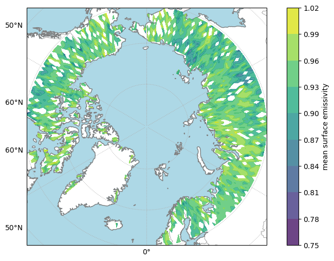

Summary

🎉 Congratulations! You’ve successfully created a cloud-native data analysis workflow.

What You Accomplished

✅ Built a virtual datacube from numerous satellite files without downloading
✅ Created a ~12MB reference file representing GB+ of data
✅ Analyzed and visualized satellite data directly from cloud storage
✅ Learned transferable skills for other cloud-hosted datasets

Next Steps

Expand temporally: Add date ranges to process months/years of data
Try other missions: Apply to MODIS, GOES, or other NASA datasets
Add parallel processing: Use Dask for distributed computing
Share your work: Export reference files for collaborators

Resources

📚 Kerchunk documentation • VirtualiZarr tutorials • NASA Earthdata Cloud