import os
from pathlib import Path

import cartopy.crs as ccrs
import earthaccess
import h5py
import numpy as np
import PIL
from matplotlib import pyplot as pltMOPITT Carbon Monoxide (CO) Mixing Ratio
Summary
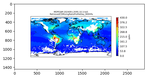
This code makes a GIF from the RetrievedCOMixingRatioProfileDay variable from Measurements Of Pollution In The Troposphere (MOPITT).
Prerequisites
A free(!) account at https://www.earthdata.nasa.gov/ is needed to login and download the appropriate files.
This notebook was tested last using Python 3.10.15, and requires these libraries:
1. Setup
2. Search for data using earthaccess
We use earthaccess to streamline the login to NASA Earthdata.
Additional resources about earthaccess
earthaccess.login()<earthaccess.auth.Auth at 0x103e4f160>short_name = "MOP03JM"
version = "9"
results = earthaccess.search_data(
short_name=short_name,
version=version,
provider="LARC_CLOUD", # this is needed only temporary, while there are still non-LARC_CLOUD versions of these granules.
temporal=("2024-09", "2024-10"),
)
print(f"{len(results)} file(s) found.")2 file(s) found.print(results)[Collection: {'ShortName': 'MOP03JM', 'Version': '9'}
Spatial coverage: {'HorizontalSpatialDomain': {'Geometry': {'BoundingRectangles': [{'WestBoundingCoordinate': -180.0, 'EastBoundingCoordinate': 180.0, 'NorthBoundingCoordinate': 90.0, 'SouthBoundingCoordinate': -90.0}]}}}
Temporal coverage: {'RangeDateTime': {'BeginningDateTime': '2024-09-01T00:00:04.694Z', 'EndingDateTime': '2024-09-01T23:59:59.999Z'}}
Size(MB): 146.863
Data: ['https://data.asdc.earthdata.nasa.gov/asdc-prod-protected/MOPITT/MOP03JM.9/2024.09.01/MOP03JM-202409-L3V95.10.3.he5'], Collection: {'ShortName': 'MOP03JM', 'Version': '9'}
Spatial coverage: {'HorizontalSpatialDomain': {'Geometry': {'BoundingRectangles': [{'WestBoundingCoordinate': -180.0, 'EastBoundingCoordinate': 180.0, 'NorthBoundingCoordinate': 90.0, 'SouthBoundingCoordinate': -90.0}]}}}
Temporal coverage: {'RangeDateTime': {'BeginningDateTime': '2024-10-01T00:00:05.832Z', 'EndingDateTime': '2024-10-01T23:59:59.999Z'}}
Size(MB): 149.263
Data: ['https://data.asdc.earthdata.nasa.gov/asdc-prod-protected/MOPITT/MOP03JM.9/2024.10.01/MOP03JM-202410-L3V95.10.3.he5']]3. Download data
downloaded_files = earthaccess.download(results, local_path=".")
downloaded_files
['MOP03JM-202409-L3V95.10.3.he5', 'MOP03JM-202410-L3V95.10.3.he5']4. Open the files
arrays = {"lon": [], "lat": [], "CO_mixing_ratio": []}

# Open and read file
for i, file in enumerate(downloaded_files):
    with h5py.File(file, mode="r") as f:
        # Slice data to get the pressure level of your choice
        #   [Longitude(Xdim):360 , Latitude(Ydim):180, Presure level:9]
        #   Pressure Level: 0 = 900 hPa, 1 = 800 hPa, 2 = 700 hPa, 3 = 600 hPa
        #   4 = 500 hPa, 5 = 400 hpa, 6 = 300 hPa, 7 = 200 hPa, 8 = 100 hPa
        data = f["/HDFEOS/GRIDS/MOP03/Data Fields/RetrievedCOMixingRatioProfileDay"][:]
        data = np.transpose(data)

        # Retrieve the lat and lon data as well as the area of your choice
        lon = f["/HDFEOS/GRIDS/MOP03/Data Fields/Longitude"][:]
        lat = f["/HDFEOS/GRIDS/MOP03/Data Fields/Latitude"][:]

        # Turn the -9999.0 into a NaN
        masked_data = np.ma.masked_where(data <= 0, data)
        CO_mixing_ratio = data.copy()
        CO_mixing_ratio[masked_data <= 0] = np.nan

        arrays["lon"].append(lon)
        arrays["lat"].append(lat)
        arrays["CO_mixing_ratio"].append(CO_mixing_ratio)
5. Generate plots
pressure_levels = np.arange(0, 9)

proj = ccrs.PlateCarree()

for file_index, file in enumerate(downloaded_files):
    filestem = Path(file).stem
    os.makedirs(filestem, exist_ok=True)

    # Plot all graphs.
    for i in pressure_levels:
        fig, ax = plt.subplots(figsize=(7.20, 3.60), dpi=80, subplot_kw={"projection": proj})

        im = ax.contourf(
            arrays["lon"][file_index],
            arrays["lat"][file_index],
            arrays["CO_mixing_ratio"][file_index][i, :, :],
            levels=np.linspace(0, 430, 25),
            cmap="jet",
            vmin=0,
            vmax=430,
            transform=proj,
        )
        ax.coastlines()

        cb = plt.colorbar(im, shrink=0.76)
        cb.set_label("ppbv", fontsize=8)

        pressure_prefix = -i + 9
        plt.title(
            f"{file}\n RetrievedCOMixingRatioProfileDay_{str(pressure_prefix)}00hPa", fontsize=8
        )

        # Save the figure.
        name_prefix = f"{filestem}/{filestem}_RetrievedCOMixingRatioProfileDay"
        plt.savefig(f"{name_prefix}_{pressure_prefix}00hPa.jpg", dpi=400)
        print(f"Plot has been saved: {name_prefix}_{pressure_prefix}00hPa.jpg")
        plt.close()
Plot has been saved: MOP03JM-202409-L3V95.10.3/MOP03JM-202409-L3V95.10.3_RetrievedCOMixingRatioProfileDay_900hPa.jpg
Plot has been saved: MOP03JM-202409-L3V95.10.3/MOP03JM-202409-L3V95.10.3_RetrievedCOMixingRatioProfileDay_800hPa.jpg
Plot has been saved: MOP03JM-202409-L3V95.10.3/MOP03JM-202409-L3V95.10.3_RetrievedCOMixingRatioProfileDay_700hPa.jpg
Plot has been saved: MOP03JM-202409-L3V95.10.3/MOP03JM-202409-L3V95.10.3_RetrievedCOMixingRatioProfileDay_600hPa.jpg
Plot has been saved: MOP03JM-202409-L3V95.10.3/MOP03JM-202409-L3V95.10.3_RetrievedCOMixingRatioProfileDay_500hPa.jpg
Plot has been saved: MOP03JM-202409-L3V95.10.3/MOP03JM-202409-L3V95.10.3_RetrievedCOMixingRatioProfileDay_400hPa.jpg
Plot has been saved: MOP03JM-202409-L3V95.10.3/MOP03JM-202409-L3V95.10.3_RetrievedCOMixingRatioProfileDay_300hPa.jpg
Plot has been saved: MOP03JM-202409-L3V95.10.3/MOP03JM-202409-L3V95.10.3_RetrievedCOMixingRatioProfileDay_200hPa.jpg
Plot has been saved: MOP03JM-202409-L3V95.10.3/MOP03JM-202409-L3V95.10.3_RetrievedCOMixingRatioProfileDay_100hPa.jpg
Plot has been saved: MOP03JM-202410-L3V95.10.3/MOP03JM-202410-L3V95.10.3_RetrievedCOMixingRatioProfileDay_900hPa.jpg
Plot has been saved: MOP03JM-202410-L3V95.10.3/MOP03JM-202410-L3V95.10.3_RetrievedCOMixingRatioProfileDay_800hPa.jpg
Plot has been saved: MOP03JM-202410-L3V95.10.3/MOP03JM-202410-L3V95.10.3_RetrievedCOMixingRatioProfileDay_700hPa.jpg
Plot has been saved: MOP03JM-202410-L3V95.10.3/MOP03JM-202410-L3V95.10.3_RetrievedCOMixingRatioProfileDay_600hPa.jpg
Plot has been saved: MOP03JM-202410-L3V95.10.3/MOP03JM-202410-L3V95.10.3_RetrievedCOMixingRatioProfileDay_500hPa.jpg
Plot has been saved: MOP03JM-202410-L3V95.10.3/MOP03JM-202410-L3V95.10.3_RetrievedCOMixingRatioProfileDay_400hPa.jpg
Plot has been saved: MOP03JM-202410-L3V95.10.3/MOP03JM-202410-L3V95.10.3_RetrievedCOMixingRatioProfileDay_300hPa.jpg
Plot has been saved: MOP03JM-202410-L3V95.10.3/MOP03JM-202410-L3V95.10.3_RetrievedCOMixingRatioProfileDay_200hPa.jpg
Plot has been saved: MOP03JM-202410-L3V95.10.3/MOP03JM-202410-L3V95.10.3_RetrievedCOMixingRatioProfileDay_100hPa.jpg6. Create gif
frames = []
pressures = np.arange(1, 10)[::-1]

for file in downloaded_files:
    filestem = Path(file).stem
    name_prefix = f"{filestem}/{filestem}_RetrievedCOMixingRatioProfileDay"

    for j in pressures:
        new_frame = PIL.Image.open(rf"{name_prefix}_{j}00hPa.jpg")
        frames.append(new_frame)
        frames[0].save(
            f"{name_prefix}_PressureLevels.gif",
            format="GIF",
            append_images=frames[:],
            save_all=True,
            duration=250,
            loop=0,
            quality=75,
            optimize=True,
        )

    print(f"GIF has been saved: {name_prefix}_PressureLevels.gif")
GIF has been saved: MOP03JM-202409-L3V95.10.3/MOP03JM-202409-L3V95.10.3_RetrievedCOMixingRatioProfileDay_PressureLevels.gif
GIF has been saved: MOP03JM-202410-L3V95.10.3/MOP03JM-202410-L3V95.10.3_RetrievedCOMixingRatioProfileDay_PressureLevels.gif# Display first frame of gif in notebook for illustration purposes.
import matplotlib.image as mpimg
img = mpimg.imread(f"{name_prefix}_PressureLevels.gif")
plt.imshow(img)