Note
Go to the end to download the full example code.
Configuring Models
At times, model templates need to be parametrized in a more of a programming sense than a mathematical one. An example of this is a linear time invariant (LTI) ODE system, where the size of the state vector and whether there is feedback control are dependent on what the user passes in for the state and input matrices.
Module Configuration
One option for generating models is through a settings object in the top-level
condor name space, where you register the module’s default configuration with
get_settings. Then the module is imported via get_module.
Here is the configured model source with the name _lti.py:
 1import numpy as np
 2
 3import condor
 4
 5# pass get_settings in a list of configurable variables with defaults
 6# it returns a dictionary with the the configured values
 7conf = condor.settings.get_settings(A=np.array([1.0]), B=None)
 8A, B = conf.values()
 9
10
11class LTI(condor.ODESystem):
12    x = state(shape=A.shape[0])
13
14    xdot = A @ x
15
16    if B is not None:
17        K = parameter(shape=B.T.shape)
18
19        u = -K @ x
20        dynamic_output.u = u
21
22        xdot += B @ u
23
24    dot[x] = xdot
To use this module, we use get_module(), passing its declared
settings as concrete keyword arguments.
The returned object is a module, so we can access the model with its declared class name:
LTI_dblint = dblint_mod.LTI
And finally we can use this configured ODE system to simulate a trajectory.
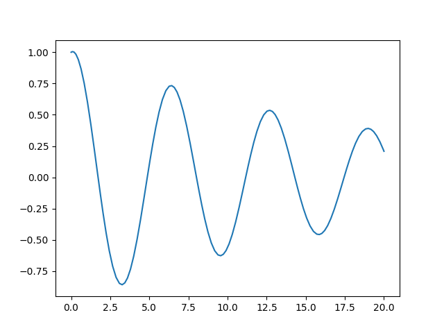
[<matplotlib.lines.Line2D object at 0x7fdce0a5c920>]
We can also re-use the module with a different configuration:
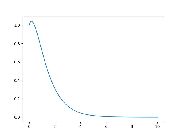
[<matplotlib.lines.Line2D object at 0x7fdce09d7890>]
Programmatic Construction
An alternative approach is to programmatically generate the model using the metaprogramming machinery Condor uses internally. See Metaprogramming class declaration for a more thorough overview.
from condor.contrib import ModelTemplateType, ODESystem


def make_LTI(A, B=None, name="LTISystem"):
    attrs = ModelTemplateType.__prepare__(name, (ODESystem,))

    attrs["A"] = A

    state = attrs["state"]
    x = state(shape=A.shape[0])
    attrs["x"] = x

    xdot = A @ x

    if B is not None:
        attrs["B"] = B
        K = attrs["parameter"](shape=B.T.shape)
        attrs["K"] = K

        u = -K @ x
        attrs["dynamic_output"].u = u

        xdot += B @ u

    attrs["dot"][x] = xdot

    plant = ModelTemplateType(name, (ODESystem,), attrs)

    return plant

    # OR for primary models:
    ode_attrs = condor.ODESystem.__prepare__(ode_name, (condor.ODESystem,))
    ode_model = condor.ODESystem.__class__(ode_name, (condor.ODESystem,), ode_attrs)

    # but submodels must be ~ the way shown above:
    event_meta_args = (
        event_name,
        (ode_model.Event, condor.models.Submodel),
    )
    event_attrs = condor.contrib.Event.__prepare__(*event_meta_args)
    condor.contrib.EventType.__new__(
        condor.contrib.EventType,
        *event_meta_args,
        attrs=event_attrs,
    )
Use of the model factory function looks similar to using get_module:

[<matplotlib.lines.Line2D object at 0x7fdce0b81eb0>]
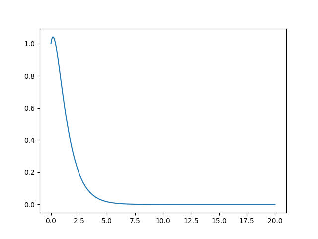
[<matplotlib.lines.Line2D object at 0x7fdce0a828d0>]
plt.show()
Total running time of the script: (0 minutes 0.419 seconds)