Discrete Time LQR

import numpy as np
from _sgm_test_util import LTI_plot
from matplotlib import pyplot as plt

import condor as co


class DblIntSampled(co.ODESystem):
    A = np.array([[0.0, 1.0], [0.0, 0.0]])
    B = np.array([[0.0], [1.0]])

    K = parameter(shape=(1, B.shape[0]))
    dt = parameter()

    x = state(shape=A.shape[0])
    u = state(shape=B.shape[1])

    dot[x] = A @ x + B @ u

To implement the periodic sampling, we use an event with at_time with a slice specification, starting at time 0 and occurring every dt time units without end.

class SampleEvent(DblIntSampled.Event):
    at_time = slice(None, None, dt)

    update[u] = -K @ x

Now declare the trajectory analysis to simulate

class DblIntSampledLQR(DblIntSampled.TrajectoryAnalysis):
    tf = 32.0

    initial[x] = [1.0, 0.1]
    # can initialize for aesthetics, but zero-crossing at t=0 updates it
    initial[u] = -K @ initial[x]

    Q = np.eye(2)
    R = np.eye(1)

    cost = trajectory_output(integrand=(x.T @ Q @ x + u.T @ R @ u) / 2)

    class Options:
        adjoint_adaptive_max_step_size = False
        state_max_step_size = 0.5 / 8
        adjoint_max_step_size = 0.5 / 8


dt = 0.5
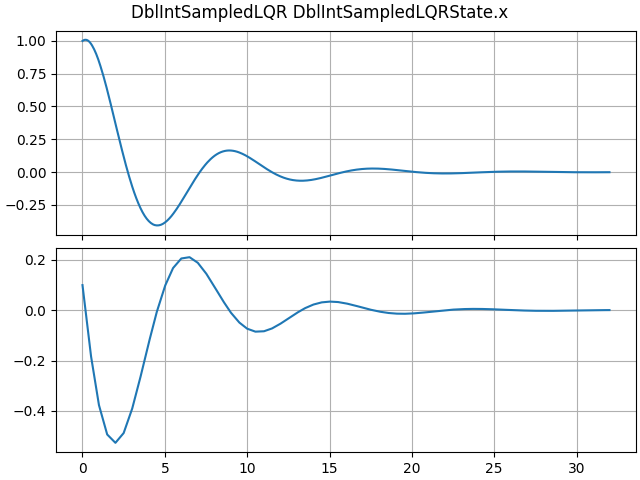
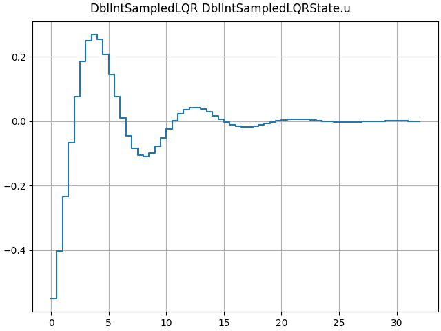
sim = DblIntSampledLQR(K=[0.5, 0.5], dt=dt)
LTI_plot(sim)

• 
• 

Determine the optimal gain by embedding the trajectory analysis in an optimization problem:

class SampledOptLQR(co.OptimizationProblem):
    K = variable(shape=DblIntSampledLQR.K.shape)
    params = parameter.create_from(DblIntSampled.parameter, K=K)
    sim = DblIntSampledLQR(**params)
    objective = sim.cost

    class Options:
        __implementation__ = co.implementations.ScipyCG


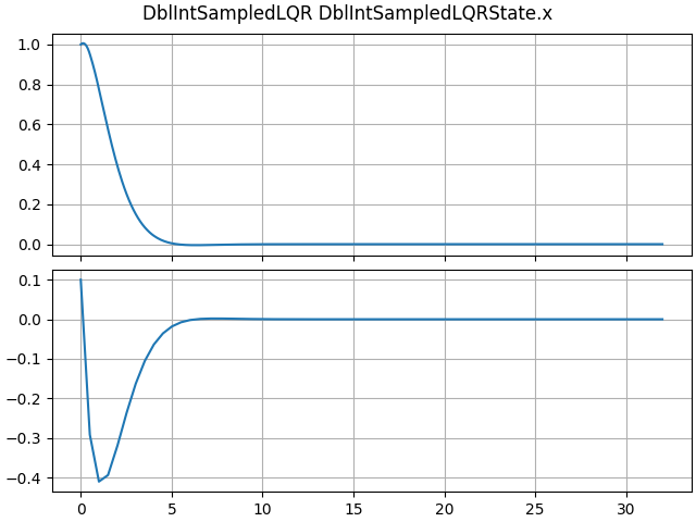
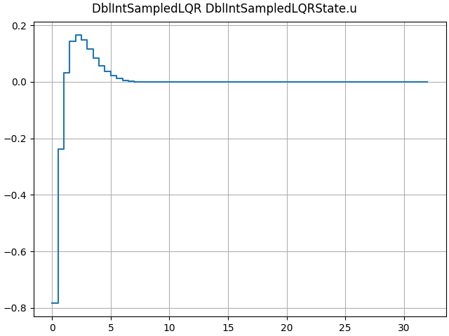
lqr_sol = SampledOptLQR(dt=dt)

print(lqr_sol.K)

/opt/hostedtoolcache/Python/3.12.11/x64/lib/python3.12/site-packages/condor/implementations/iterative.py:481: RuntimeWarning: Method CG cannot handle bounds.
  min_out = minimize(
[[0.66131423 1.32662666]]

Compare with the solution from the discrete algebraic Riccati equation:

from scipy import linalg, signal

Ad, Bd, _, _, _ = signal.cont2discrete(
    (DblIntSampledLQR.A, DblIntSampledLQR.B, None, None), dt
)
S = linalg.solve_discrete_are(Ad, Bd, DblIntSampledLQR.Q, DblIntSampledLQR.R)
K = linalg.solve(Bd.T @ S @ Bd + DblIntSampledLQR.R, Bd.T @ S @ Ad)

print(K)

[[0.65140165 1.31420219]]

sim_are = DblIntSampledLQR(K=K, dt=dt)
LTI_plot(sim_are)

• 
• 

plt.show()