Optimal Transfer With State Trigger

from time import perf_counter

import matplotlib.pyplot as plt
import numpy as np
from _sgm_test_util import LTI_plot

import condor as co


class DblInt(co.ODESystem):
    A = np.array([[0, 1], [0, 0]])
    B = np.array([[0], [1]])

    x = state(shape=A.shape[0])
    mode = state()

    p1 = parameter()
    p2 = parameter()

    u = modal()

    dot[x] = A @ x + B * u


class Accel(DblInt.Mode):
    condition = mode == 0.0
    action[u] = 1.0


class Switch1(DblInt.Event):
    function = x[0] - p1
    update[mode] = 1.0


class Decel(DblInt.Mode):
    condition = mode == 1.0
    action[u] = -1.0


class Switch2(DblInt.Event):
    function = x[0] - p2
    # update[mode] = 2.
    terminate = True


from scipy.optimize import bisect


class Transfer(DblInt.TrajectoryAnalysis):
    initial[x] = [-9.0, 0.0]
    xd = [1.0, 2.0]
    Q = np.eye(2)
    cost = trajectory_output(((x - xd).T @ (x - xd)) / 2)
    tf = 20.0

    class Options:
        rootfinder = bisect
        rootfinder_xtol = 1e-15


p0 = -4.0, -1.0
sim = Transfer(*p0)
# sim.implementation.callback.jac_callback(sim.implementation.callback.p, [])

class MinimumTime(co.OptimizationProblem):
    p1 = variable()
    p2 = variable()
    sim = Transfer(p1, p2)
    objective = sim.cost

    class Options:
        # exact_hessian = False
        __implementation__ = co.implementations.ScipyCG


MinimumTime.set_initial(p1=p0[0], p2=p0[1])

t_start = perf_counter()
opt = MinimumTime()
t_stop = perf_counter()

print("time to run:", t_stop - t_start)
print(opt.p1, opt.p2)
print(opt._stats)

/opt/hostedtoolcache/Python/3.12.12/x64/lib/python3.12/site-packages/condor/implementations/iterative.py:484: RuntimeWarning: Method CG cannot handle bounds.
  min_out = minimize(
time to run: 0.21667061400000875
[-3.00000001] [1.]
 message: Optimization terminated successfully.
 success: True
  status: 0
     fun: 1.5050883330650572e-17
       x: [-3.000e+00  1.000e+00]
     nit: 6
     jac: [-3.168e-09  1.554e-14]
    nfev: 14
    njev: 14

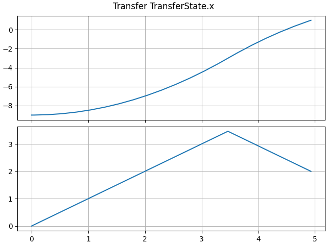
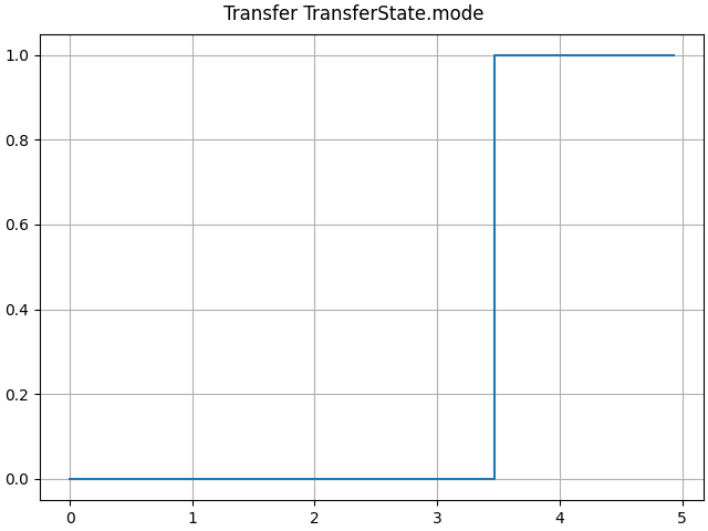
Original result:

axes = LTI_plot(opt.sim)

• 
• 

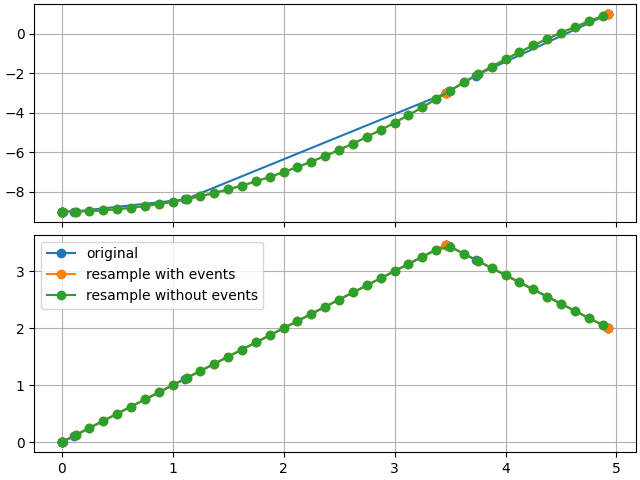
Comparing resampling results

sim_1 = opt.sim.resample(0.125)
sim_2 = opt.sim.resample(0.125, include_events=False)
sim_3 = sim_1.resample(0.125, include_events=False)

# resample always calls the original simulation result to have full fidelity
assert np.all(sim_2._res.x == sim_3._res.x)

plotting utilities

def plot_x(axes, sim, label):
    for ax, x in zip(axes, sim.x):
        ax.plot(sim.t, x.squeeze(), "o-", label=label)


def make_figure():
    fig, axes = plt.subplots(2, constrained_layout=True, sharex=True)
    for ax in axes:
        ax.grid(True)

    plot_x(axes, opt.sim, "original")
    plot_x(axes, sim_1, "resample with events")
    plot_x(axes, sim_2, "resample without events")
    plt.legend()
    return axes

In this case, we actually up-sampled

axes = make_figure()

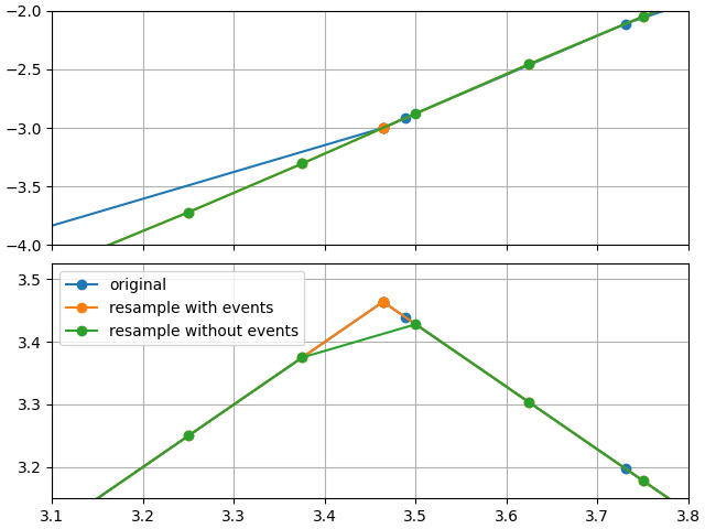
looking near the first event trigger, we see the impact of re-sampling without events

axes = make_figure()
plt.xlim(3.1, 3.8)
axes[0].set_ylim(-4, -2)
axes[1].set_ylim(3.15, 3.525)
plt.show()