Working with trajectories

Condor is not intended to be an optimal control library per se, but we often end up working with trajectories a great deal and spent considerable effort to make modeling dynamical systems nice.

Glider Model

For this tutorial, we will consider a simplified model of a glider with some form of angle-of-attack control. We can represent this as a system of ordinary differential equations (ODEs) given by

$$\begin{array}{r}\begin{array}{rl}\dot{r}& =v\cos \gamma \\ \dot{h}& =v\sin \gamma \\ \dot{\gamma }& =(CL(\alpha )\cdot v^2-g\cos \gamma )/v\\ \dot{v}& =-CD(\alpha )\cdot v^2-g\sin \gamma \end{array}\end{array}$$

where $r$ is the range, or horizontal position, $h$ is the altitude, or vertical position, $v$ is the velocity, $\gamma$ is the flight-path angle, and $\alpha$ is the angle-of-attack, which modulates the coefficients of lift, $CL$, and drag, $CD$, and $g$ is the acceleration due to gravity. Simple models of the lift and drag are given by

$$\begin{array}{r}\begin{array}{rl}CL(\alpha )& =C{L}_{\alpha }\cdot \alpha \\ CD(\alpha )& =C{D}_0+C{D}_{i,q}\cdot C{L}^2\end{array}\end{array}$$

where $C{L}_{\alpha }$ is the lift slope, $C{D}_0$ is the 0-lift drag, and $C{D}_{i,q}$ is the quadratic coefficient for the lift-induced drag. In Condor, we can implement this as,

import condor
from condor.backend import operators as ops


class Glider(condor.ODESystem):
    r = state()
    h = state()
    gamma = state()
    v = state()

    alpha = modal()

    CL_alpha = parameter()
    CD_0 = parameter()
    CD_i_q = parameter()
    g = parameter()

    CL = CL_alpha * alpha
    CD = CD_0 + CD_i_q * CL**2

    dot[r] = v * ops.cos(gamma)
    dot[h] = v * ops.sin(gamma)
    dot[gamma] = (CL * v**2 - g * ops.cos(gamma)) / v
    dot[v] = -CD * v**2 - g * ops.sin(gamma)

    initial[r] = 0.0
    initial[h] = 1.0
    initial[v] = 15.0
    initial[gamma] = 30 * ops.pi / 180.0

The modal field is used to define elements with deferred and possibly varying behavior, so we use this for the angle-of-attack so we can simulate multiple behaviors. To simulate this model, we create a TrajectoryAnalysis, a sub-model to an ODE Sysstem, which is ultimately responsible for defining the specifics of integrating the ODE. In this example, the TrajectoryAnalysis model only specifies the final simulation time of the model. It is more mathematically consistent to have the initial values defined in the trajectory analysis, but for convenience we declared it as part of the ODE system.

class FirstSim(Glider.TrajectoryAnalysis):
    tf = 20.0

The fields of the original Glider simulation are copied to the TrajectoryAnalysis so the parameter values must be supplied to evaluate the model numerically.

A = 3e-1
first_sim = FirstSim(CL_alpha=0.11 * A, CD_0=0.05 * A, CD_i_q=0.05, g=1.0)

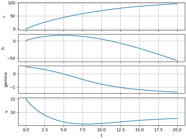
In addition to binding static parameters like the other built-in models, the time-histories for the state and dynamic_output are bound and can be accessed for plotting. For example, we can plot time histories

from matplotlib import pyplot as plt

state_data = first_sim.state.asdict()

fig, axs = plt.subplots(nrows=len(state_data), constrained_layout=True, sharex=True)
for ax, (state_name, state_hist) in zip(axs, state_data.items()):
    ax.plot(first_sim.t, state_hist)
    ax.set_ylabel(state_name)
    ax.grid(True)
ax.set_xlabel("t")

Text(0.5, 18.167, 't')

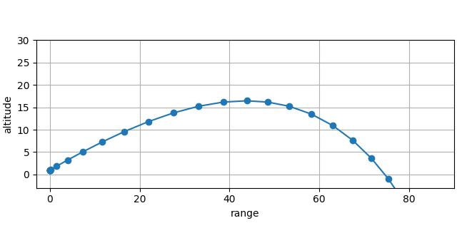
and the flight path

import numpy as np


def flight_path_plot(sims, **plot_kwargs):
    fig, ax = plt.subplots(constrained_layout=True, figsize=(6.4, 3.2))
    plt.ylabel("altitude")
    plt.xlabel("range")
    # reverse zorders to show progression of sims more nicely
    zorders = np.linspace(2.1, 2.5, len(sims))[::-1]
    marker = plot_kwargs.pop("marker", "o")
    for sim, zorder in zip(sims, zorders):
        ax.plot(sim.r, sim.h, marker=marker, zorder=zorder, **plot_kwargs)
    plt.grid(True)
    ax.set_aspect("equal")
    ax.set_ylim(-3, 30)
    ax.set_xlim(-3, 90)
    return ax


flight_path_plot([first_sim])

<Axes: xlabel='range', ylabel='altitude'>

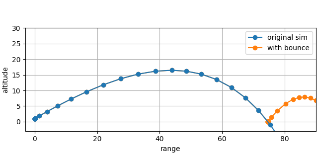
Modeling the Ground with an Event

Notice the glider eventually flies straight through the ground. We can fix that with an Event sub-model that detects the altitude zero-crossing and flips the descent to an ascent with a simple parametrized loss model.

class Bounce(Glider.Event):
    function = h
    update[gamma] = -gamma
    mu = parameter()
    update[v] = mu * v

We still need to create a new TrajectoryAnalysis since the FirstSim was bound to the Glider model at the time of creation (without the bounce event).

class BounceSim(Glider.TrajectoryAnalysis):
    tf = 20.0


bounce_sim = BounceSim(**first_sim.parameter.asdict(), mu=0.9)

flight_path_plot([first_sim, bounce_sim])
plt.legend(["original sim", "with bounce"])

<matplotlib.legend.Legend object at 0x7f65b59051f0>

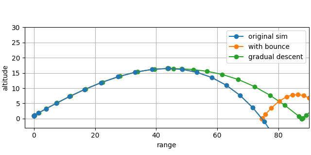
Angle of Attack Control with a Mode

We can also add a behavior for the angle of attack using a mode, in this case holding a constant angle of attack after reaching peak altitude to reduce rate of descent.

To ensure proper numerical behavior, we follow [orbital ref] and use an accumulator state to encode the flight controller logic. In this case, we create an event to detect the switch from ascent to descent and perform a state update.

class MaxAlt(Glider.Event):
    function = gamma
    max_alt = state()
    update[max_alt] = h

The mode can now be triggered by the accumulator state update, where we set $\alpha$ to a new constant parameter.

class DescentAlphaHold(Glider.Mode):
    condition = max_alt > 0
    hold_alpha = parameter()
    action[alpha] = hold_alpha

The glider now travels a little further with this control behavior.

class AlphaSim(Glider.TrajectoryAnalysis):
    tf = 20.0


alpha_sim = AlphaSim(**bounce_sim.parameter.asdict(), hold_alpha=0.5)

ax = flight_path_plot([first_sim, bounce_sim, alpha_sim])
ax.legend(["original sim", "with bounce", "gradual descent"])

<matplotlib.legend.Legend object at 0x7f65b5997a40>

Trajectory Outputs

So far, we have only used the TrajectoryAnalysis to simulate the ODE System. In order to use the ODE system as part of other condor models, we must declare trajectory_output. Condor computes the gradient of the trajectory_output using the Sweeping Gradient method. Each trajectory output has the form

$$J=\varphi (t_f,x\left(t_f\right),p)+{\int }_{t_0}^{t_f}L(\tau ,x\left(\tau \right),p)d\tau$$

where $\varphi$ is the terminal term, $L(\cdot )$ is the integrand term, and $x\left(t\right)$ is the solution to the system of ODEs with events and modes.

First we’ll change the control behavior to use a constant angle of attack through the whole trajectory to get the peak altitude to vary. We’ll also make the bounce event terminal since we’re interested in the flown range.

class ConstantAlphaHold(Glider.Mode):
    condition = 1
    action[alpha] = 1 * DescentAlphaHold.hold_alpha


Bounce.terminate = True

We can form the area under the flight-path curve by taking the derivative $\dot{r}$ and using it to form the integrand. We can also just take the final max altitude state we added with the MaxAlt event and the final range.

class AlphaSim(Glider.TrajectoryAnalysis):
    initial[r] = 0.0
    initial[h] = 1.0
    initial[v] = 15.0
    initial[gamma] = 30 * ops.pi / 180.0
    tf = 100.0

    area = trajectory_output(integrand=dot[r] * h)
    max_h = trajectory_output(max_alt)
    max_r = trajectory_output(r)

    class Options:
        state_rtol = 1e-12
        state_atol = 1e-15
        adjoint_rtol = 1e-12
        adjoint_atol = 1e-15

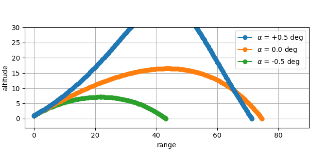
Then we can compare areas with different hold angles of attack:

params = bounce_sim.parameter.asdict()
results = {
    "alpha = +0.5 deg": AlphaSim(**params, hold_alpha=0.5),
    "alpha = 0.0 deg": AlphaSim(**params, hold_alpha=0.0),
    "alpha = -0.5 deg": AlphaSim(**params, hold_alpha=-0.5),
}

print(*[f"{k}: {v.area}" for k, v in results.items()], sep="\n")

alpha = +0.5 deg: [1459.42002699]
alpha = 0.0 deg: [825.36407495]
alpha = -0.5 deg: [214.23621474]

ax = flight_path_plot(results.values())
ax.legend([k.replace("alpha", r"$\alpha$") for k in results])

<matplotlib.legend.Legend object at 0x7f65b4758710>

Embedding

With several trajectory_output elements declared, we can embed the trajectory within other Condor models, for example to maximize a combination of the peak height and flown range.

class GlideOpt(condor.OptimizationProblem):
    alpha = variable(
        initializer=0.001,
        lower_bound=-1.0,
        upper_bound=1,
        warm_start=False,
    )
    sim = AlphaSim(**bounce_sim.parameter.asdict(), hold_alpha=alpha)
    trade_off = parameter()
    objective = -(trade_off * sim.max_h + (1 - trade_off) * sim.max_r)

    class Options:
        exact_hessian = False
        print_level = 0
        tol = 1e-3
        max_iter = 8


opt_range = GlideOpt(trade_off=0)

ax = flight_path_plot([opt_range.sim])
ax.text(
    *(0.05, 0.92),
    f"max range: {opt_range.sim.max_r} ($\\alpha={opt_range.alpha}$",
    transform=ax.transAxes,
)

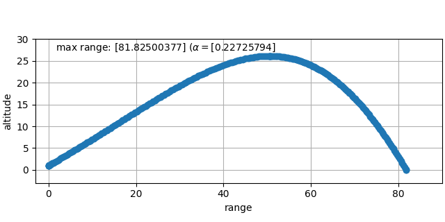
Text(0.05, 0.92, 'max range: [81.82500377] ($\\alpha=[0.22725794]$')

We can store the iteration history using iter_callback option on OptimizationProblem, pointing it to the method of a class to store the simulation data on each call. Since it only gets information relevant to the optimization problem itself, we use from_values() to reconstruct the internals of the analysis with the simulation outputs bound to the sim attribute.

class IterStore:
    def __init__(self):
        self.parameter = None

    def init_callback(self, parameter, impl_opts):
        self.parameter = parameter
        self.iters = []

    def iter_callback(self, i, variable, objective, constraint):
        iter_opt_res = GlideOpt.from_values(
            **variable.asdict(),
            **self.parameter.asdict(),
        )
        self.iters.append(iter_opt_res)


hist = IterStore()
GlideOpt.Options.init_callback = hist.init_callback
GlideOpt.Options.iter_callback = hist.iter_callback

opt_alt = GlideOpt(trade_off=1)

ax = flight_path_plot([it.sim for it in hist.iters], marker=None)
ax.legend([f"iter {idx}, alpha={sim.alpha}" for idx, sim in enumerate(hist.iters)])
ax.set_title("max altitude iterations")
ax.set_ylim(-3, 45)

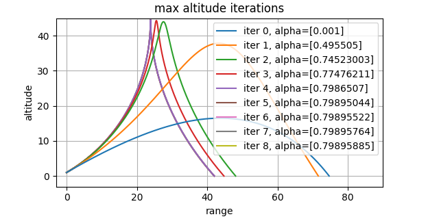
(-3.0, 45.0)