Tabular Data

It is often useful to interpolate pre-existing data. For this, the TableLookup model provides a convenient way to specify the interpolant input and output data. This model also provids an example of using a ExternalSolverWrapper by wrapping uses the ndsplines library to perform the interpolation and compute derivatives as needed for tensor-product B-splines. Note that this table model assumes fixed input and output data, but a model with variable input and output data could be defined as needs arise.

Because TableLookup is an ExternalSolverWrapper, the declaration of a model quite different from a standard ModelTemplate, with the relevant data is passed in in a way that appears more similar to a standard Python object instantiation with arguments for the input data, output data, degree, and boundary conditions. Condor supports any number of inputs, and automatically computes the derivatives \(\frac{dy_i}{dx_j}\) as needed.

Basic Usage

Here we demonstrate the construction of a single-input, single-output table for the \(sin\) function

import numpy as np

import condor
from condor.backend import operators as ops

# input and output data are dictionaries with keys for the name of the element and
# values to construct the interpolant.
data_x = dict(x=np.linspace(-1, 1, 5) * ops.pi)
data_y = dict(y=ops.sin(data_x["x"]))
SinTable = condor.TableLookup(data_x, data_y)


out = SinTable(np.pi / 2)
print(out.y)
assert np.isclose(out.y, 1)

[1.]

Multiple Inputs

Next, we construct a table with two inputs and a single output. The output data should have shape (n_x1, n_x2, ...)

Table = condor.TableLookup(
    dict(
        x1=[-1, -0.5, 0, 0.5, 1],
        x2=[0, 1, 2, 3],
    ),
    dict(
        y1=[
            [0, 1, 2, 3],
            [3, 4, 5, 6],
            [6, 7, 8, 9],
            [8, 7, 6, 5],
            [4, 3, 2, 1],
        ]
    ),
)

tab_out = Table(x1=0.5, x2=0.1)
print(tab_out.output)

TableLookupOutput(y1=array([7.62482755]))

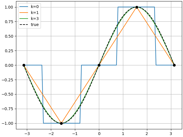
Spline Degree and Boundary Conditions

Next we demonstrate specifying the degrees (and boundary conditions) for the SinTable. Note that these can be specified for each input (and boundary) independently, or a single custom value can be broadcast to each input (and boundary).

from matplotlib import pyplot as plt

eval_x = np.linspace(-1.1, 1.1, 100) * np.pi

fig, ax = plt.subplots(constrained_layout=True)
for k in [0, 1, 3]:
    # for cubic polynomial, use constant slope (constant first derivative, 0 second
    # derivative) boundary condition instead of default not-a-knot (constant, non-zero,
    # second derivative)
    bcs = (2, 0) if k == 3 else (-1, 0)

    SinTable = condor.TableLookup(data_x, data_y, degrees=k, bcs=bcs)
    y = np.array([SinTable(x).y for x in eval_x]).squeeze()

    plt.plot(eval_x, y, label=f"k={k}")

plt.plot(data_x["x"], data_y["y"], "ko")
plt.plot(eval_x, np.sin(eval_x), "k--", label="true")

plt.grid(True)
plt.legend()

plt.show()