Continuous Time LQR

import matplotlib.pyplot as plt
import numpy as np
from _sgm_test_util import LTI_plot

import condor as co


class DblInt(co.ODESystem):
    A = np.array([[0.0, 1.0], [0.0, 0.0]])
    B = np.array([[0.0], [1.0]])

    K = parameter(shape=(1, B.shape[0]))

    x = state(shape=A.shape[0])
    dynamic_output.u = -K @ x

    dot[x] = A @ x + B @ u


class DblIntLQR(DblInt.TrajectoryAnalysis):
    tf = 32.0

    initial[x] = [1.0, 0.1]

    Q = np.eye(2)
    R = np.eye(1)

    cost = trajectory_output(integrand=(x.T @ Q @ x + u.T @ R @ u) / 2)

    class Options:
        state_rtol = 1e-8
        adjoint_rtol = 1e-8


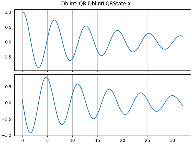
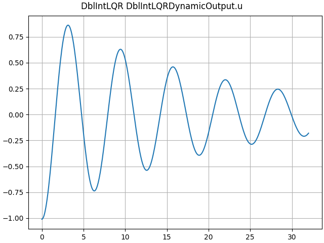
ct_sim = DblIntLQR(K=[1.0, 0.1])
LTI_plot(ct_sim)

• 
• 

Determine the optimal gain by embedding the trajectory analysis in an optimization problem:

class CtOptLQR(co.OptimizationProblem):
    K = variable(shape=DblIntLQR.K.shape)

    sim = DblIntLQR(K=K)
    objective = sim.cost

    class Options:
        __implementation__ = co.implementations.ScipyCG


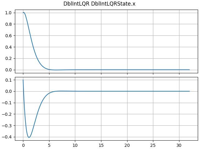
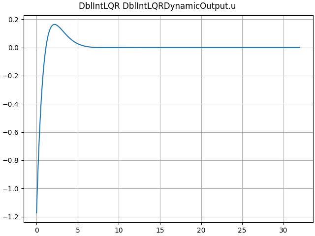
lqr_sol = CtOptLQR()

print(lqr_sol.K)

/opt/hostedtoolcache/Python/3.12.11/x64/lib/python3.12/site-packages/condor/implementations/iterative.py:481: RuntimeWarning: Method CG cannot handle bounds.
  min_out = minimize(
[[0.99997598 1.73199404]]

Compare with the solution from the continuous algebraic Riccati equation:

from scipy import linalg

S = linalg.solve_continuous_are(DblIntLQR.A, DblIntLQR.B, DblIntLQR.Q, DblIntLQR.R)
K = linalg.solve(DblIntLQR.R, DblIntLQR.B.T @ S)

print(K)

[[1.         1.73205081]]

sim_are = DblIntLQR(K=K)
LTI_plot(sim_are)

• 
• 

plt.show()