Optimal Transfer With Time Trigger

from time import perf_counter

import matplotlib.pyplot as plt
import numpy as np
from _sgm_test_util import LTI_plot

import condor as co

# either include time as state or increase tolerances to ensure sufficient ODE solver
# accuracy
with_time_state = False

Define the double integrator system

class DblInt(co.ODESystem):
    A = np.array([[0, 1], [0, 0]])
    B = np.array([[0], [1]])

    x = state(shape=A.shape[0])
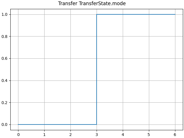
    mode = state()
    u = modal()

    dot[x] = A @ x + B * u

    if with_time_state:
        tt = state()
        dot[tt] = 1.0

Now a mode to accelerate

class Accel(DblInt.Mode):
    condition = mode == 0.0
    action[u] = 1.0

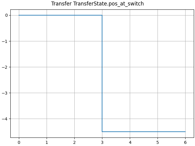
An event to switch to deceleration, specified by a paramter \(t_1\). We’ll also create a state to capture the position at the switch event.

class Switch1(DblInt.Event):
    t1 = parameter()
    pos_at_switch = state()

    at_time = t1
    update[mode] = 1.0
    update[pos_at_switch] = x[0]

Now the mode to switch to deceleration, triggered by Switch1 updating the mode.

class Decel(DblInt.Mode):
    condition = mode == 1.0
    action[u] = -1.0

Finally a terminating event specified by a new parameter \(t_2\).

class Switch2(DblInt.Event):
    t2 = parameter()
    at_time = Switch1.t1 + t2
    terminate = True

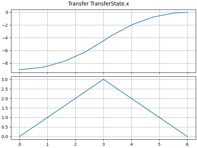
The trajectory analysis adds a terminal quadratic cost for error with respect to the desired final position \((0, 0)\).

class Transfer(DblInt.TrajectoryAnalysis):
    initial[x] = [-9.0, 0.0]
    Q = np.eye(2)
    cost = trajectory_output((x.T @ Q @ x) / 2)

    if not with_time_state:

        class Options:
            state_adaptive_max_step_size = 4


sim = Transfer(t1=1.0, t2=4.0)
print(sim.pos_at_switch)
# jac = sim.implementation.callback.jac_callback(sim.implementation.callback.p, [])

[ 0.   0.   0.   0.   0.   0.   0.   0.   0.   0.   0.   0.  -8.5 -8.5
 -8.5 -8.5 -8.5 -8.5 -8.5 -8.5]

Now embed the trajectory analysis in an optimization to minimize the final position error over transfer and final times.

class MinimumTime(co.OptimizationProblem):
    t1 = variable(lower_bound=0)
    t2 = variable(lower_bound=0)
    transfer = Transfer(t1, t2)
    objective = transfer.cost

    class Options:
        # exact_hessian = False
        __implementation__ = co.implementations.ScipyCG


"""
old:
eval jacobian for jac_Transfer
args [DM([1, 4]), DM(00)]
p=[1, 4]
[[-56.9839, 0]]



"""

'\nold:\neval jacobian for jac_Transfer\nargs [DM([1, 4]), DM(00)]\np=[1, 4]\n[[-56.9839, 0]]\n\n\n\n'

MinimumTime.set_initial(t1=2.163165480675697, t2=4.361971866705403)

t_start = perf_counter()
opt = MinimumTime()
t_stop = perf_counter()

print("time to run:", t_stop - t_start)
print(opt.t1, opt.t2)
# print(jac)
print(opt._stats)

/opt/hostedtoolcache/Python/3.12.11/x64/lib/python3.12/site-packages/condor/implementations/iterative.py:481: RuntimeWarning: Method CG cannot handle bounds.
  min_out = minimize(
time to run: 0.3653668100000118
[2.99999968] [2.99999216]
 message: Optimization terminated successfully.
 success: True
  status: 0
     fun: 3.008671708973335e-11
       x: [ 3.000e+00  3.000e+00]
     nit: 12
     jac: [-4.048e-06 -7.514e-06]
    nfev: 22
    njev: 22

LTI_plot(opt.transfer)

• 
• 
• 

Another version of the transfer analysis excluding the switch event.

class AccelerateTransfer(DblInt.TrajectoryAnalysis, exclude_events=[Switch1]):
    initial[x] = [-9.0, 0.0]
    Q = np.eye(2)
    cost = trajectory_output((x.T @ Q @ x) / 2)

    if not with_time_state:

        class Options:
            state_adaptive_max_step_size = 4


# TODO?
# class AccelerateTransfer(Transfer, exclude_events=[Switch1]):
#     pass

sim_accel = AccelerateTransfer(**opt.transfer.parameter.asdict())
assert sim_accel._res.e[0].rootsfound.size == opt.transfer._res.e[0].rootsfound.size - 1  # noqa

plt.show()