2 Working with EMIT L2A Reflectance and NEON L3 Directional Reflectance Data

Summary

In the previous notebook Finding Co-located EMIT and NEON AOP Data, we found and downloaded co-located EMIT L2A Reflectance and NEON L3 Airborne Reflectance data over the NEON Niwot Ridge site in Colorado. In this notebook, we will open and explore both datasets to better understand the structure of the data from these two sensors, then we will conduct some common preprocessing routines to work with the data together, including applying quality data information relevant to each sensor, cropping, and interactive visualization.

Background

The EMIT instrument is an imaging spectrometer that measures light in visible and infrared wavelengths. These measurements display unique spectral signatures that correspond to the composition on the Earth’s surface. The EMIT mission focuses specifically on mapping the composition of minerals to better understand the effects of mineral dust throughout the Earth system and human populations now and in the future. In addition, the EMIT instrument can be used in other applications, such as mapping of greenhouse gases, snow properties, and water resources.

More details about EMIT and its associated products can be found on the EMIT website and EMIT product pages hosted by the LP DAAC.

The NEON Imaging Spectrometer (NIS) is an airborne imaging spectrometer built by JPL (AVIRIS-NG) and operated by the National Ecological Observatory Network’s (NEON) Airborne Observation Platform (AOP). NEON’s hyperspectral sensors collect measurements of sunlight reflected from the Earth’s surface in 426 narrow (~5 nm) spectral channels spanning wavelengths between ~ 380 - 2500 nm. NEON’s remote sensing data is intended to map and answer questions about a landscape, with ecological applications including identifying and classifying plant species and communities, mapping vegetation health, detecting disease or invasive species, and mapping droughts, wildfires, or other natural disturbances and their impacts.

NEON surveys sites spanning the Continental US, Alaska, Hawaii, and Puerto Rico, during peak phenological greenness, capturing each site 3 out of every 5 years, for most terrestrial sites (*Hawaii and Puerto Rico are surveyed ~1 out of every 4-5 years). AOP’s Flight Schedules and Coverage provides more information about current and past airborne schedules.

More detailed information about NEON’s airborne sampling design can be found in the paper: Spanning scales: The airborne spatial and temporal sampling design of the National Ecological Observatory Network.

References
- Leith, Alex. 2023. Hyperspectral Notebooks. Jupyter Notebook. Auspatious. https://github.com/auspatious/hyperspectral-notebooks/tree/main - Musinsky et al. 2022. Spanning Scales: the airborne spatial and temporal sampling design o the National Ecological Observatory Network.

Requirements
- NASA Earthdata Account
- No Python setup requirements if connected to the workshop cloud instance!
- Local Only Set up Python Environment - See setup_instructions.md in the /setup/ folder to set up a local compatible Python environment
- Downloaded necessary files. This is done at the end of the 01_Finding_Co-located_NEON_EMIT_Data_NIWO notebook.

Learning Objectives
- Open and work with EMIT L2A Reflectance and NEON L3 Hyperspectral Reflectance data
- Apply a quality mask to EMIT datasets
- Crop EMIT data - Interactively explore reflectance spectra

Tutorial Outline

1 Setup
2 Opening and Exploring EMIT Reflectance Data
2.1 Applying Quality Masks to EMIT Data
2.2 Interactive Spectral Plots
2.3 Cropping EMIT Data
2.4 Output cropped EMIT dataset to a netcdf file
3 Opening and Exploring NEON Reflectance Data
3.1 Convert AOP h5 reflectance to xarray dataset 3.2 Interactive Spatial Plots 3.3 Interactive Spectral Plots

1 Setup

This tutorial is the 2nd tutorial in a series. Make sure you have downloaded the EMIT and NEON datasets into the expected folders, following the previous tutorial: Finding Co-located EMIT and NEON AOP Data.

After downloading the data, import Python libraries.

# Import Packages
import os
import math
import numpy as np
import xarray as xr
import h5py
from osgeo import gdal
import rasterio as rio
import rioxarray as rxr
import hvplot.xarray
import hvplot.pandas
import holoviews as hv
import geopandas as gp
import cartopy.crs as ccrs
import geopandas as gp

from vitals.emit_tools import emit_xarray
import geoviews as gv
#from holoviews.plotting.links import DataLink

Define a filepath for an EMIT L2A Reflectance file and EMIT L2A Mask file. These were downloaded in the previous tutorial. The files selected in this example are from June 25, 2023.

emit_fp = "../../data/emit_refl/EMIT_L2A_RFL_001_20230625T170814_2317611_005.nc"
emit_qa_fp = "../../data/emit_refl/EMIT_L2A_MASK_001_20230625T170814_2317611_005.nc"

2 Opening and Exploring EMIT Reflectance Data

EMIT L2A Reflectance Data are distributed in a non-orthocorrected spatially raw NetCDF4 (.nc) format consisting of the data and its associated metadata. Inside the L2A Reflectance .nc file there are 3 groups. Groups can be thought of as containers to organize the data.

The root group that can be considered the main dataset contains the reflectance data described by the downtrack, crosstrack, and bands dimensions.
The sensor_band_parameters group containing the wavelength center and the full-width half maximum (FWHM) of each band.
The location group contains latitude and longitude values at the center of each pixel described by the crosstrack and downtrack dimensions, as well as a geometry lookup table (GLT) described by the ortho_x and ortho_y dimensions. The GLT is an orthorectified image (EPSG:4326) consisting of 2 layers containing downtrack and crosstrack indices. These index positions allow us to quickly project the raw data onto this geographic grid.

To work with the EMIT data, we will use the emit_tools module. There are other ways to work with the data and a more thorough explanation of the emit_tools in the EMIT-Data-Resources Repository.

Open the example EMIT scene using the emit_xarray function. In this step we will use the ortho=True argument to orthorectify the scene using the included GLT.

emit_ds = emit_xarray(emit_fp, ortho=True)
emit_ds

emit_ds.coords['spatial_ref']

<xarray.DataArray 'spatial_ref' ()> Size: 8B
array(0)
Coordinates:
    spatial_ref  int64 8B 0
Attributes:
    crs_wkt:                      GEOGCS["WGS 84",DATUM["WGS_1984",SPHEROID["...
    semi_major_axis:              6378137.0
    semi_minor_axis:              6356752.314245179
    inverse_flattening:           298.257223563
    reference_ellipsoid_name:     WGS 84
    longitude_of_prime_meridian:  0.0
    prime_meridian_name:          Greenwich
    geographic_crs_name:          WGS 84
    horizontal_datum_name:        World Geodetic System 1984
    grid_mapping_name:            latitude_longitude
    spatial_ref:                  GEOGCS["WGS 84",DATUM["WGS_1984",SPHEROID["...

We can plot the spectra of an individual pixel closest to a latitude and longitude we want using the sel function from xarray. Using the good_wavelengths flag from the sensor_band_parameters group, mask out bands where water absorption features were assigned a value of -0.01 reflectance. Typically data around 1320-1440 nm and 1770-1970 nm is noisy due to the moisture present in the atmosphere; therefore, these spectral regions offer little information about targets and can be excluded from calculations.

emit_ds['reflectance'].data[:,:,emit_ds['good_wavelengths'].data==0] = np.nan

Now select a point and plot a spectra. In this example, we’ll first find the center of the scene and use those coordinates.

scene_center = emit_ds.latitude.values[int(len(emit_ds.latitude)/2)],emit_ds.longitude.values[int(len(emit_ds.longitude)/2)]
scene_center

(np.float64(40.00857386925845), np.float64(-105.69955918991546))

point = emit_ds.sel(latitude=scene_center[0],longitude=scene_center[1], method='nearest')
point.hvplot.line(y='reflectance',x='wavelengths', color='black').opts(
    title=f'Latitude = {point.latitude.values.round(3)}, Longitude = {point.longitude.values.round(3)}')

We can also plot individual bands spatially by selecting a wavelength, then plotting. First mask out fill_values introduced during the orthorectification process by assigning their values to nan. Then select the band with a wavelengths of 850 nm and plot it using ESRI imagery as a basemap to get a better picture of the scene.

emit_ds['reflectance'].data[emit_ds['reflectance'].data == -9999] = np.nan

emit_layer = emit_ds.sel(wavelengths=850,method='nearest')
emit_layer.hvplot.image(rasterize=True, dynamic=False, cmap='viridis',geo=True, tiles='ESRI', crs='EPSG:4326', frame_width=720,frame_height=405, alpha=0.7, fontscale=2).opts(
    title=f"{emit_layer.wavelengths:.3f} {emit_layer.wavelengths.units}", xlabel='Longitude',ylabel='Latitude')

2.1 Applying Quality Masks to EMIT Data

The EMIT L2A Mask file contains some bands that are direct masks (Cloud, Dilated, Cirrus, Water, Spacecraft), and some (AOD550 and H2O (g cm-2)) that contain information calculated during the L2A reflectance retrieval. These may be used as additional screening, depending on the application. The Aggregate Flag is the mask used during EMIT L2B Mineralogy calculations, which we will also use here, but not all users might want this particular mask.

Note: It is more memory efficient to apply the mask before orthorectifying, the automation section in the EMIT notebooks show how to do that.

emit_mask = emit_xarray(emit_qa_fp, ortho=True)
emit_mask

# optionally look at the info
# emit_mask.info()

List the quality flags contained in the mask_bands dimension.

emit_mask.mask_bands.data.tolist()

['Cloud flag',
 'Cirrus flag',
 'Water flag',
 'Spacecraft Flag',
 'Dilated Cloud Flag',
 'AOD550',
 'H2O (g cm-2)',
 'Aggregate Flag']

As mentioned, we will use the Aggregate Flag. First mask areas with fill_value of -9999 like we did for reflectence, then select the Aggregate Flag band with the sel function as we did for wavelengths before.

emit_mask['mask'].data[emit_mask['mask'].data == -9999] = np.nan

emit_aggregate_mask = emit_mask.sel(mask_bands='Aggregate Flag')

Now we can visualize our aggregate quality mask. You may have noticed before that we added a lot of parameters to our plotting function. If we want to consistently apply the same formatting for multiple plots, we can add those arguments to a dictionary that we can unpack into hvplot functions using **.

Create two dictionaries with plotting options.

size_opts = dict(frame_height=405, frame_width=720, fontscale=2)
map_opts = dict(geo=True, crs='EPSG:4326', alpha=0.7, xlabel='Longitude',ylabel='Latitude')

emit_aggregate_mask.hvplot.image(rasterize=True, dynamic=False, cmap='viridis', tiles='ESRI', **size_opts, **map_opts)

Values of 1 in the mask indicate areas to omit. Apply the mask to our EMIT Data by assigning values where the mask.data == 1 to np.nan

emit_ds.reflectance.data[emit_aggregate_mask.mask.data == 1] = np.nan

We can confirm our masking worked with a spatial plot.

emit_layer_filtered_plot = emit_ds.sel(wavelengths=850, method='nearest').hvplot.image(rasterize=True, dynamic=False, cmap='viridis',tiles='ESRI',**size_opts, **map_opts)
emit_layer_filtered_plot

2.2 Interactive Spectral Plots

Combining the Spatial and Spectral information into a single visualization can be a powerful tool for exploring and inspecting imaging spectroscopy data. Using the streams module from Holoviews we can link a spatial map to a plot of spectra.

We could plot a single band image as we previously have, but using a multiband image, like an RGB may help infer what targets we’re examining. Build an RGB image following the steps below.

Select bands to represent red (650 nm), green (560 nm), and blue (470 nm) by finding the nearest to a wavelength chosen to represent that color.

emit_rgb = emit_ds.sel(wavelengths=[650, 560, 470], method='nearest')

We may need to adjust balance the brightness of the selected wavelengths to make a prettier map. This will not affect the data, just the visuals. To do this we will use the function below. We can change the bright argument to increase or decrease the brightness of the scene as a whole. A value of 0.2 usually works pretty well.

def gamma_adjust(rgb_ds, bright=0.2, white_background=False):
    array = rgb_ds.reflectance.data
    gamma = math.log(bright)/math.log(np.nanmean(array)) # Create exponent for gamma scaling - can be adjusted by changing 0.2 
    scaled = np.power(np.nan_to_num(array,nan=1),np.nan_to_num(gamma,nan=1)).clip(0,1) # Apply scaling and clip to 0-1 range
    if white_background == True:
        scaled = np.nan_to_num(scaled, nan = 1) # Set NANs to 1 so they appear white in plots
    rgb_ds.reflectance.data = scaled
    return rgb_ds

emit_rgb = gamma_adjust(emit_rgb, white_background=True)

Now that we have an RGB dataset, we can use that to create a spatial plot, and data selected by clicking on that ‘map’ can be inputs for a function to return values from the full dataset at that latitude and longitude location using the cell below. To visualize the spectral and spatial data side-by-side, we use the Point Draw tool from the holoviews library.

Define a limit to the quantity of points and spectra we will plot, a list of colors to cycle through, and an initial point. Then use the input from the Tap function to provide clicked x and y positions on the map and use these to retrieve spectra from the dataset at those coordinates.

Click in the RGB image to add spectra to the plot. You can also click and hold the mouse button then drag previously place points. To remove a point click and hold the mouse button down, then press the backspace key.

# Interactive Spectral/Spatial Plotting
# Modified from https://github.com/auspatious/hyperspectral-notebooks/blob/main/03_EMIT_Interactive_Points.ipynb

# Starting Point from center pixel
x_start = scene_center[1]
y_start = scene_center[0]

# Set Point Limit
POINT_LIMIT = 10

# Set up Color Cycling
color_cycle = hv.Cycle('Category20')

# Define initial point and spatial plot
first_point = ([x_start], [y_start], [0])
points = gv.Points(first_point, kdims=['longitude','latitude'], vdims='id', crs=ccrs.PlateCarree())

# Define Point Draw Plot
points_stream = hv.streams.PointDraw(
    data=points.columns(),
    source=points,
    drag=True,
    num_objects=POINT_LIMIT,
    styles={'fill_color': color_cycle.values[:POINT_LIMIT], 'line_color': 'gray'}
)

# RGB Plot without Basemap
rgb_map = emit_rgb.hvplot.rgb(x='longitude', y='latitude', bands='wavelengths',
                            frame_height=480, frame_width=480,
                            crs=ccrs.PlateCarree(),
                            title="Stretched RGB EMIT Image")
# Set up tap and point streams
posxy = hv.streams.PointerXY(source=rgb_map, x=x_start, y=y_start)
clickxy = hv.streams.Tap(source=rgb_map, x=x_start, y=y_start)

# Function to build spectral plot of clicked location to show on hover stream plot
def click_spectra(data):
    coordinates = [c for c in zip(data['longitude'], data['latitude'])]
    
    plots = {}
    for i, coords in enumerate(coordinates):
        x, y = coords
        selected = emit_ds['reflectance'].sel(longitude=x, latitude=y, method="nearest")
        plots[i] = (
            selected.hvplot.line(
                y="reflectance",
                x="wavelengths",
                label=f"{i}"
            )
        )
        points_stream.data["id"][i] = i
    return hv.NdOverlay(plots).opts(hv.opts.Curve(color=color_cycle))
    
# Function to provide hover spectra
def hover_spectra(x,y):
    return emit_ds['reflectance'].sel(longitude=x,latitude=y,method='nearest').hvplot.line(y='reflectance',x='wavelengths',
                                                                           color='black', frame_width=480)
# Define the Dynamic Maps
click_dmap = hv.DynamicMap(click_spectra, streams=[points_stream])
hover_dmap = hv.DynamicMap(hover_spectra, streams=[posxy])

# Plot the Map and Dynamic Map side by side
hv.Layout(hover_dmap*click_dmap + rgb_map * points).cols(2).opts(
    hv.opts.Points(active_tools=['point_draw'], size=10, tools=['hover'], color='white', line_color='gray'),
    hv.opts.Overlay(show_legend=False, show_title=False, fontscale=1.5, frame_height=480)
)

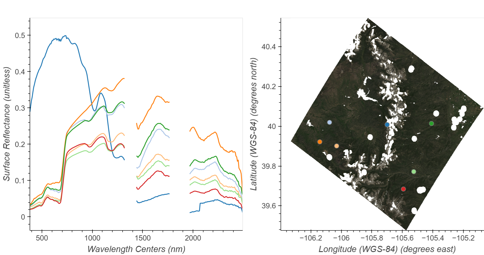
We can take these selected points and the corresponding reflectance spectra and save them as a .csv for later use.

Select 10 points by adding to the figure above. We will save these and use them in a to calculate Equivalent Water Thickness or Canopy water content in the next notebook.

Build a dictionary of the selected points and spectra, then export the spectra to a .csv file.

data = points_stream.data
wavelengths = emit_ds.wavelengths.values

rows = [["id", "longitude", "latitude"] + [str(i) for i in wavelengths]]
 
for p in zip(data['longitude'], data['latitude'], data['id']):
    x, y, i = p
    spectra = emit_ds.sel(longitude=x, latitude=y, method="nearest").reflectance.values
    row = [i, x, y] + list(spectra)
    rows.append(row)

We’ve preselected 10 points, but feel free to uncomment the cell below to use your own. This will overwrite the file containing the preselected points.

# with open('../data/emit_click_data.csv', 'w', newline='') as f:
#     writer = csv.writer(f)
#     writer.writerows(rows)

2.3 Cropping EMIT data to a Region of Interest

To crop our dataset to our ROI, we first need to open a shapefile of the region. Open the downloaded shapefile of all AOP flight boxes, filter to the Niwot Ridge site (NIWO) and plot it onto the EMIT 850nm reflectance spatial plot. To ensure proper georeferencing of the EMIT scene, be sure to specify the CRS (this is done for the image in the map_opts dictionary).

aop_flightboxes = gp.read_file("../../data/AOP_flightBoxes/AOP_flightboxesAllSites.shp")
niwo_polygon = aop_flightboxes[aop_flightboxes.siteID == 'NIWO']
shape = niwo_polygon

emit_ds.sel(wavelengths=850, method='nearest').hvplot.image(rasterize=True, dynamic=False, cmap='viridis',**size_opts,**map_opts,tiles='ESRI')*shape.hvplot(color='#FFFF00',alpha=0.5, crs='EPSG:4326')

Now use the clip function from rasterio to crop the data to our ROI using our shape’s geometry and crs. The all_touched=True argument will ensure all pixels touched by our polygon will be included.

emit_cropped = emit_ds.rio.clip(shape.geometry.values,shape.crs, all_touched=True)

Plot the cropped data.

emit_cropped.sel(wavelengths=850,method='nearest').hvplot.image(rasterize=True, dynamic=False, cmap='viridis', tiles='ESRI', **size_opts, **map_opts)

# Create RGB Map of the cropped dataset
emit_rgb_cropped = emit_cropped.sel(wavelengths=[650, 560, 470], method='nearest')
emit_rgb_cropped = gamma_adjust(emit_rgb_cropped,white_background=True)
emit_rgb_cropped.hvplot.rgb(rasterize=True, dynamic=False, fontscale=1.5, xlabel='Longitude',ylabel='Latitude',title = 'EMIT RGB Image over Niwot Ridge AOP Flight Box',geo = True, frame_width = 600) #frame_width=560, frame_height=480)

2.4 Output cropped EMIT dataset to a netcdf file

Lastly for our EMIT dataset, we can write a smaller output that we can use in later notebooks, to calculate Canopy water content or other applications. We use the granule_id from the dataset to keep a similar naming convention.

# Write Clipped Output
emit_cropped.to_netcdf(f'../../data/{emit_cropped.granule_id}_NIWO.nc')

3 NEON Hyperspectral Reflectance Data

For this example we’ll take a look at the Level-3 (1km x 1km tiled) NEON AOP directional surface bidirectional reflectance data (DP3.30006.002) that was downloaded in the previous tutorial.

3.1 Convert AOP h5 reflectance to xarray dataset

First, we’ll define a function aop_h5refl2xarray that converts AOP reflectance data from the hdf5 format into an xarray dataset so we can look at this data in a similar way to the EMIT data.

# Define a function that reads in a NEON AOP reflectance dataset and outputs an xarray object
# this function transposes and flips the data about the y axis so y coords are ascending, to match the EMIT data
def aop_h5refl2xarray(h5_filename):
    """
    Reads a NEON AOP reflectance dataset from an HDF5 file, processes it,
    and returns an xarray Dataset.

    The processing includes:
    - Transposing the data to (y, x, wavelengths) order.
    - Flipping the y-axis to ensure ascending y-coordinates.
    - Extracting reflectance data, wavelengths, FWHM, and metadata.
    - Identifying and marking bad band windows.
    - Calculating spatial coordinates (x_coords, y_coords).

    Args:
        h5_filename (str): The path to the NEON AOP HDF5 reflectance file.

    Returns:
        xr.Dataset: An xarray Dataset containing the processed reflectance data
                    and associated metadata.
    """
    # Open the HDF5 file in read mode using a 'with' statement for proper resource management.
    with h5py.File(h5_filename) as hdf5_file:
        print('Reading in ', h5_filename)

        # Extract the site name, which is typically the first key in the HDF5 file.
        sitename = list(hdf5_file.keys())[0]  
        # Access the 'Reflectance' group within the site's data.
        h5_refl_group = hdf5_file[sitename]['Reflectance']
        # Get the 'Reflectance_Data' dataset.
        refl_dataset = h5_refl_group['Reflectance_Data']
        # Load the reflectance data into a NumPy array and cast it to float32.
        refl_array = refl_dataset[()].astype('float32')

        # Transpose the array from (wavelengths, y, x) to (y, x, wavelengths)
        # to align with typical image/spatial data conventions (rows, columns, bands).
        
        # transpose so that we have y, x, wavelengths (similar to lat, lon, wavelengths)
        refl_arrayT = np.transpose(refl_array, (1, 0, 2)) 
        refl_arrayT = refl_array[::-1, :, :]  # Flip the first axis (y)

        # Get the shape of the processed reflectance array.
        refl_shape = refl_arrayT.shape
        # Extract wavelength values from the HDF5 metadata.
        wavelengths = h5_refl_group['Metadata']['Spectral_Data']['Wavelength'][:] #.astype('float32')
        # Extract Full Width at Half Maximum (FWHM) values from the HDF5 metadata.
        fwhm = h5_refl_group['Metadata']['Spectral_Data']['FWHM'][:] #.astype('float32')

        # create dictionary containing metadata information
        metadata = {}
        metadata['shape'] = refl_shape

        metadata['no_data_value'] = float(
            refl_dataset.attrs['Data_Ignore_Value'])
        metadata['scale_factor'] = float(refl_dataset.attrs['Scale_Factor'])

        # Extract the scale factor & Scale the reflectance data by the scale factor - this is memory intensive though!
        # Can do it after the fact
        # scale_factor = float(refl_dataset.attrs['Scale_Factor'])
        # refl_array = refl_array.astype(float) / scale_factor

        # Extract bad band windows
        metadata['bad_band_window1'] = (
            h5_refl_group.attrs['Band_Window_1_Nanometers'])
        metadata['bad_band_window2'] = (
            h5_refl_group.attrs['Band_Window_2_Nanometers'])

        # Initialize good_wavelengths array with 1s
        good_wavelengths = np.ones_like(wavelengths) #, dtype='float32')

        # Mark wavelengths within the bad band windows as 0
        for bad_window in [metadata['bad_band_window1'], metadata['bad_band_window2']]:
            bad_indices = np.where((wavelengths >= bad_window[0]) & (wavelengths <= bad_window[1]))[0]
            good_wavelengths[bad_indices] = 0
        good_wavelengths[-10:] = 0 # the last 10 indices also tend to be noisy
        
        # Extract metadata
        metadata['projection'] = h5_refl_group['Metadata']['Coordinate_System']['Proj4'][()].decode('utf-8')
        metadata['spatial_ref'] = h5_refl_group['Metadata']['Coordinate_System']['Coordinate_System_String'][()].decode('utf-8')
        metadata['EPSG'] = int(h5_refl_group['Metadata']
                               ['Coordinate_System']['EPSG Code'][()])

        # Parse the 'Map_Info' string to extract spatial extent information.
        # The string is split by commas to get individual components.
        map_info = str(
            h5_refl_group['Metadata']['Coordinate_System']['Map_Info'][()]).split(",")
        # extract the resolution & convert to floating decimal number
        pixel_width = float(map_info[5])
        
        pixel_height = float(map_info[6])
        # extract the upper left-hand corner coordinates from mapInfo and cast to float
        x_min = float(map_info[3]); x_min = int(x_min)
        y_max = float(map_info[4]); y_max = int(y_max)
        
        # calculate the xMax and yMin values from the dimensions
        # xMax = left edge + (# of columns * resolution)",
        x_max = x_min + (refl_shape[1]*pixel_width); x_max = int(x_max)
        # yMin = top edge - (# of rows * resolution)",
        y_min = y_max - (refl_shape[0]*pixel_height); y_min = int(y_min)

        # Calculate UTM coordinates
        x_coords = np.linspace(x_min, x_max, num=refl_shape[1]).astype(float)
        y_coordsT = np.linspace(y_min, y_max, num=refl_shape[0]).astype(float) 
        # y coords are ascending since we flipped the y in the beginning

        # Create an xarray DataArray for the reflectance data.
        # Define dimensions ('y', 'x', 'wavelengths') and coordinates.
        refl_xrT = xr.DataArray(refl_arrayT, dims=["y", "x", "wavelengths"], name="reflectance",
               coords={"y": ("y", y_coordsT), "x": ("x", x_coords),
                       "wavelengths": ("wavelengths", wavelengths), 
                       "fwhm": ("wavelengths", fwhm),
                       "good_wavelengths": ("wavelengths", good_wavelengths)})
        
        # Create the Transposed dataset
        dsT = xr.Dataset({"reflectance": refl_xrT})
              
        # Add metadata as attributes
        for key, value in metadata.items():
            if key not in ['shape', 'extent', 'ext_dict']:
                dsT.attrs[key] = value

        return dsT

h5_filepath = r"../../data/neon_refl/DP3.30006.002/neon-aop-provisional-products/2023/FullSite/D13/2023_NIWO_5/L3/Spectrometer/Reflectance/"
h5_filename = "NEON_D13_NIWO_DP3_454000_4431000_bidirectional_reflectance.h5"
aop_refl_ds = aop_h5refl2xarray(os.path.join(h5_filepath,h5_filename))

Reading in  ../../data/neon_refl/DP3.30006.002/neon-aop-provisional-products/2023/FullSite/D13/2023_NIWO_5/L3/Spectrometer/Reflectance/NEON_D13_NIWO_DP3_454000_4431000_bidirectional_reflectance.h5

os.path.join(h5_filepath,h5_filename)

'../../data/neon_refl/DP3.30006.002/neon-aop-provisional-products/2023/FullSite/D13/2023_NIWO_5/L3/Spectrometer/Reflectance/NEON_D13_NIWO_DP3_454000_4431000_bidirectional_reflectance.h5'

aop_refl_ds

# add spatial reference information to Coordinates as follows (to create an rioxarray)
aop_refl_ds.rio.write_crs(f"epsg:{aop_refl_ds.attrs['EPSG']}", inplace=True)

Next we can run a couple more pre-processing steps, of 1. scaling the reflectance data by the scale factor (NEON data are saved in an integer format, scaled by 10000, in order to save on space) 2. setting the water vapor absorption windows (defined as “bad band windows”) to NaN. Similar to the EMIT data, “good_wavelengths” are provided as one of the Coordinates in the aop_refl_ds xarray dataset, so we can use that information to keep only the valid wavelengths.

# scale by the reflectance scale factor
aop_refl_ds['reflectance'].data = aop_refl_ds['reflectance'].data/aop_refl_ds.attrs['scale_factor']

# set "bad bands" (water vapor absorption bands) to NaN
aop_refl_ds['reflectance'].data[:,:,aop_refl_ds['good_wavelengths'].data==0.0] = np.nan

aop_tile_center = aop_refl_ds.x.values[int(len(aop_refl_ds.x)/2)],aop_refl_ds.y.values[int(len(aop_refl_ds.y)/2)]
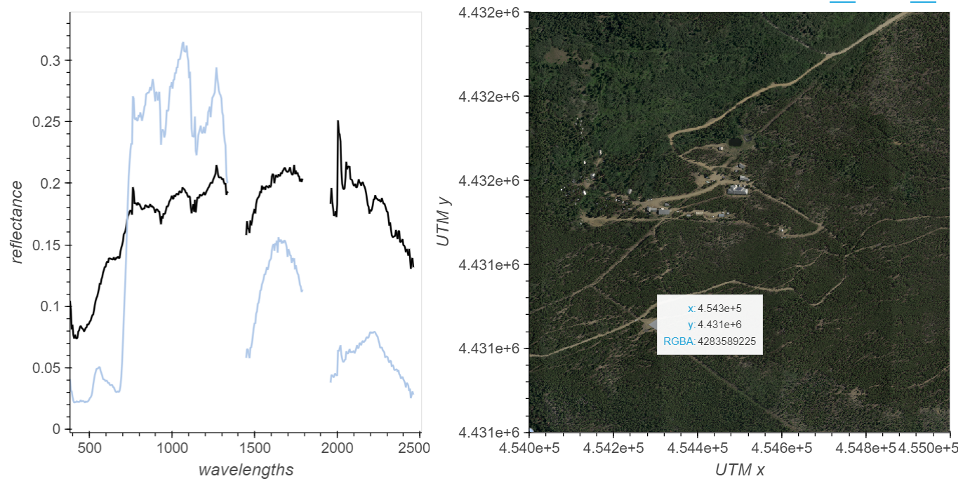
print('AOP tile center',aop_tile_center)

AOP tile center (np.float64(454500.5005005005), np.float64(4431500.5005005))

# aop_spectra = aop_refl_ds.sel(x=aop_tile_center[0],y=aop_tile_center[1], method='nearest')
aop_point = (454495,4431420) # solar panels on MRS building roof
# aop_point = aop_tile_center
aop_spectra = aop_refl_ds.sel(x=aop_point[0],y=aop_point[1], method='nearest')
aop_spectra.hvplot.line(y='reflectance',x='wavelengths', color='black').opts(
    title=f'x = {aop_spectra.x.values.round(1)}, y = {aop_spectra.y.values.round(1)}')

3.2 Interactive Spatial Plots

We can use hvplot to visualize the AOP data. The cell below allows you to visualize a single band of the AOP data for the reflectance tile, overlain on satellite imagery.

aop_refl_ds.hvplot.image(x='x',y='y',**size_opts, cmap='viridis', clim = (0,0.5), tiles='ESRI', xlabel='Longitude',ylabel='Latitude',title='NEON AOP Reflectance', crs='EPSG:4326')

# Re-project
# aop_refl_ds.rio.reproject('EPSG:4326').hvplot.image(rasterize=True, dynamic=False, x='x',y='y',**size_opts, cmap='inferno',tiles='ESRI', xlabel='Longitude',ylabel='Latitude',title='NEON AOP Reflectance', crs='EPSG:4326')

# Plot the RGB image of the NIWO tile
aop_rgb = aop_refl_ds.sel(wavelengths=[650, 560, 470], method='nearest')
aop_rgb = gamma_adjust(aop_rgb,white_background=True)
aop_rgb.hvplot.rgb(rasterize=True, dynamic=False, x='x',y='y',bands='wavelengths',xlabel='UTM x',ylabel='UTM y',title='NEON AOP Reflectance RGB',frame_width=480, frame_height=480)

3.3 Interactive Spectral Plots

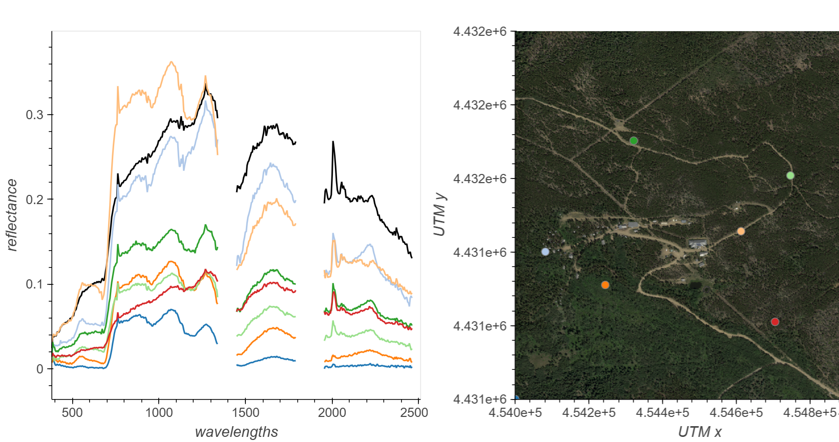
# Interactive Spectral/Spatial Plotting
# Modified from https://github.com/auspatious/hyperspectral-notebooks/blob/main/03_EMIT_Interactive_Points.ipynb

xmid = aop_refl_ds.x.values[int(len(aop_refl_ds.x) / 2)]
ymid = aop_refl_ds.y.values[int(len(aop_refl_ds.y) / 2)]
x0 = aop_refl_ds.x.values[0]
y0 = aop_refl_ds.y.values[0]

# Set Point Limit
POINT_LIMIT = 10

# Set up Color Cycling
color_cycle = hv.Cycle('Category20')

# Define initial point and spatial plot
first_point = ([x0], [y0], [0])
points = hv.Points(first_point, kdims=['x','y'], vdims='id')

# Define Point Draw Plot
points_stream = hv.streams.PointDraw(
    data=points.columns(),
    source=points,
    drag=True,
    num_objects=POINT_LIMIT,
    styles={'fill_color': color_cycle.values[:POINT_LIMIT], 'line_color': 'gray'}
)

# RGB Plot without Basemap
map = aop_rgb.hvplot.rgb(x='x',y='y',bands='wavelengths',fontscale=1.5, xlabel='UTM x',
                         ylabel='UTM y',frame_width=480, frame_height=480)

# Set up tap and point streams
posxy = hv.streams.PointerXY(source=map, x=xmid, y=ymid)
clickxy = hv.streams.Tap(source=map, x=xmid, y=ymid)

# Function to build spectral plot of clicked location to show on hover stream plot
def click_spectra(data):
    coordinates = [c for c in zip(data['x'], data['y'])]
    
    plots = {}
    for i, coords in enumerate(coordinates):
        x, y = coords
        selected = aop_refl_ds.sel(x=x, y=y, method="nearest")
        plots[i] = (
            selected.hvplot.line(
                y="reflectance",
                x="wavelengths",
                label=f"{i}"
            )
        )
        points_stream.data["id"][i] = i
    return hv.NdOverlay(plots).opts(hv.opts.Curve(color=color_cycle))
    
# Function to provide hover spectra
def hover_spectra(x,y):
    return aop_refl_ds.sel(x=x,y=y,method='nearest').hvplot.line(y='reflectance',x='wavelengths',
                                                                           color='black', frame_width=480)
# Define the Dynamic Maps
click_dmap = hv.DynamicMap(click_spectra, streams=[points_stream])
hover_dmap = hv.DynamicMap(hover_spectra, streams=[posxy])

# Plot the Map and Dynamic Map side by side
hv.Layout(hover_dmap*click_dmap + map * points).cols(2).opts(
    hv.opts.Points(active_tools=['point_draw'], size=10, tools=['hover'], color='white', line_color='gray'),
    hv.opts.Overlay(show_legend=False, show_title=False, fontscale=1.5, frame_height=480)
)

Contact Info:

Land Processes Distributed Active Archive Center (LP DAAC)¹

Email: LPDAAC@usgs.gov
Voice: +1-866-573-3222
Website: https://www.earthdata.nasa.gov/centers/lp-daac/

¹Work performed under USGS contract G15PD00467 for NASA contract NNG14HH33I.

National Ecological Observatory Network (NEON)²

Website: https://www.neonscience.org/
Contact: https://www.neonscience.org/about/contact-us

²NEON is a project sponsored by the National Science Foundation and operated by Battelle.