UQPCE

With the data files included, the user can run UQPCE using the input casefiles and compare the mean, variance, and confidence intervals with the results in this section. Files containing the data from the Monte Carlo Simulation approach will be provided upon request. These examples are included to demonstrate the use of UQPCE for varying problems.

Transonic NACA 0012 Airfoil

Background

The lift coefficient (CL) and drag coefficient (CD) of a NACA 0012 airfoil are studied in the case of transonic flight running an RANS CFD code. The inputs for the simulation are the Mach number, angle of attack (alpha), altitude, von Karman constant, and turbulent Prandtl number.

Outputs

When you execute the module, you should get results similar to those below.

Table 1 Lift coefficient PCE versus MC results.

	UQPCE	Monte Carlo
mean	0.21875	0.21875
variance	1.425e-4	1.420e-4
confidence interval	[0.1843, 0.2484]	[0.1950, 0.2412]

Table 2 Drag coefficient PCE versus MC results.

	UQPCE	Monte Carlo
mean	0.028205	0.028204
variance	1.236e-06	1.231e-06
confidence interval	[0.0253, 0.0313]	[0.0261, 0.0304]

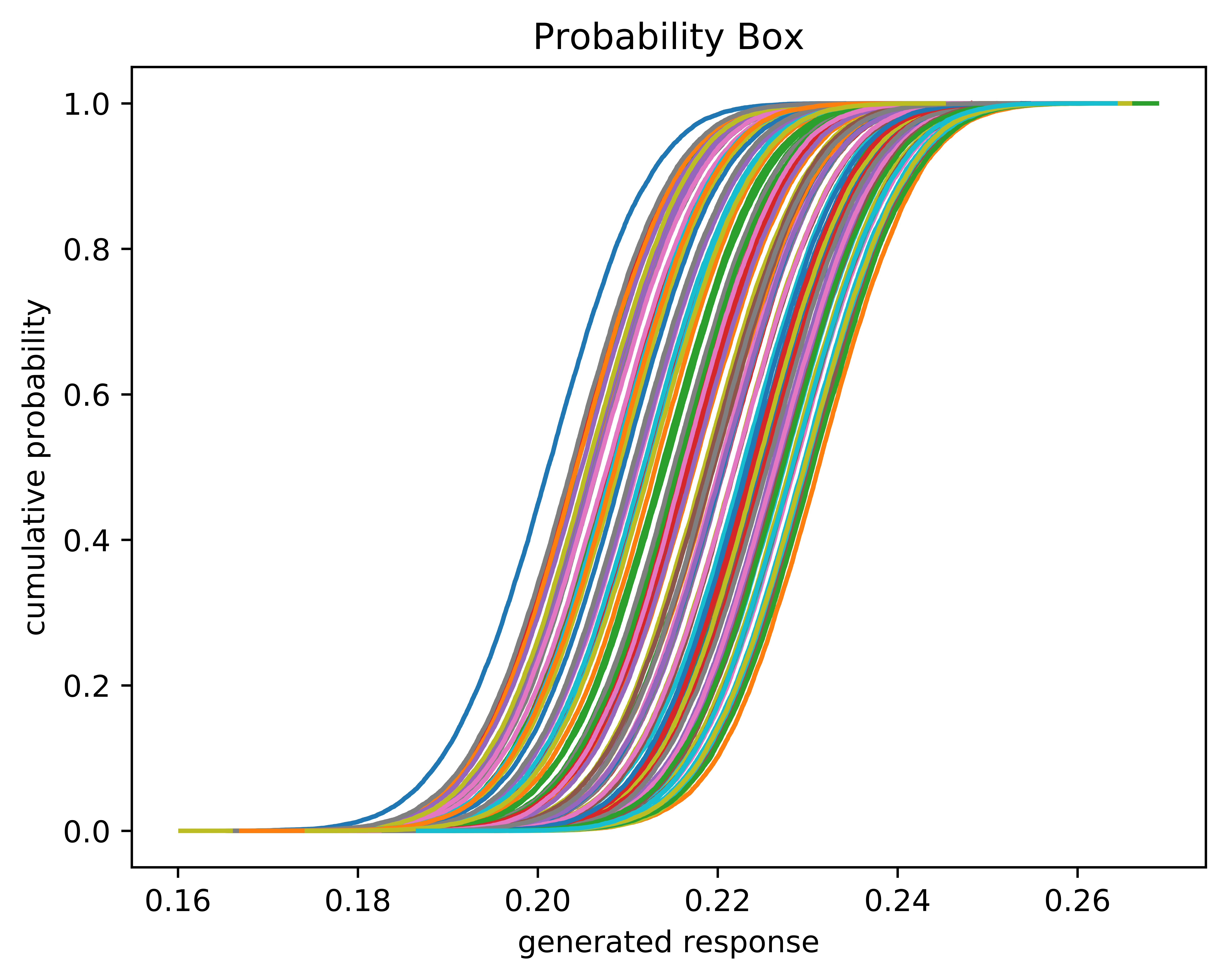
Fig. 15 The 95% confidence interval of the lift coefficient is found by interpolating to find the values that belong at 2.5% and 97.5% of the responses.

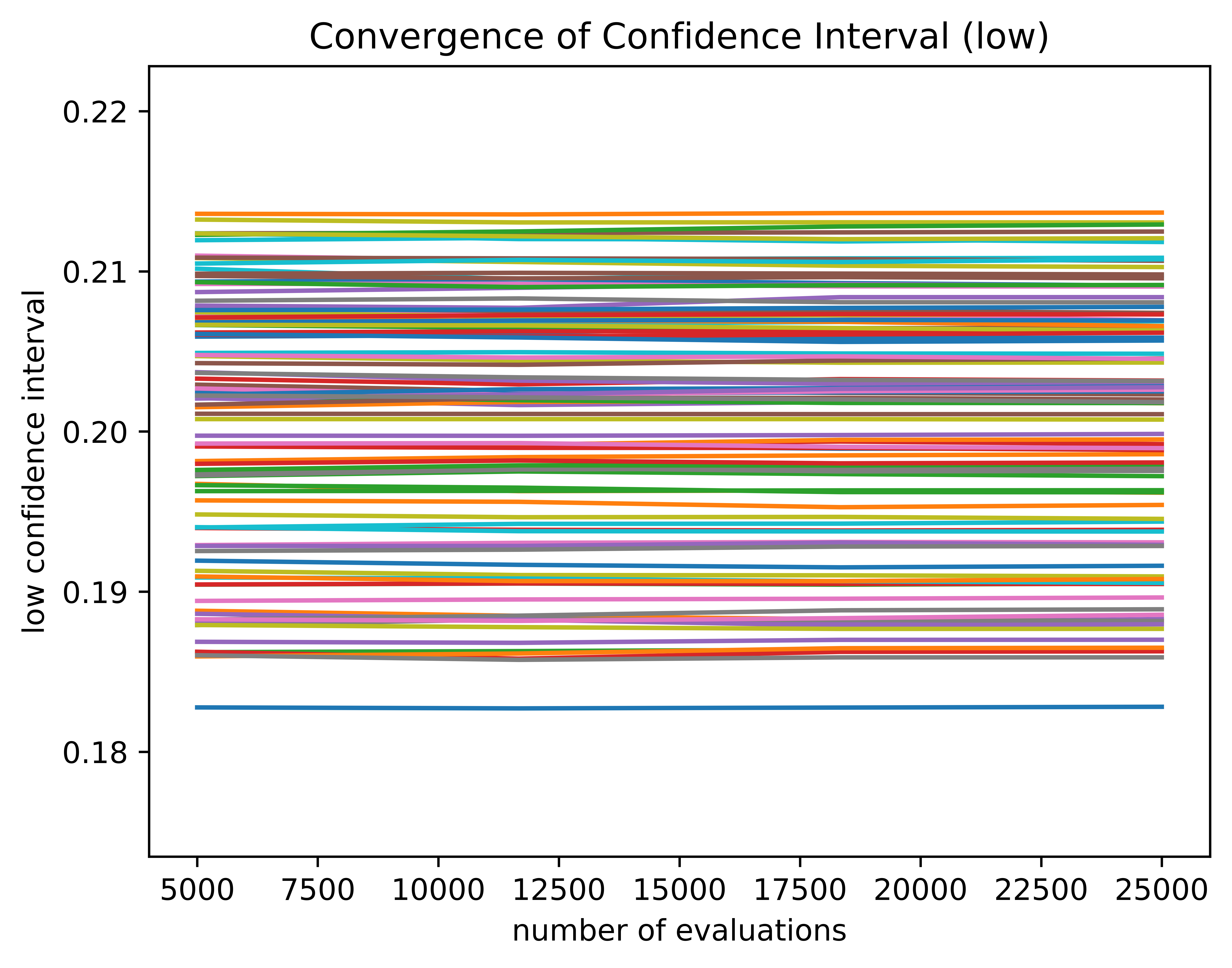
Fig. 16 The lower confidence intervals of the lift coefficient for each curve converging with additional evaluations.

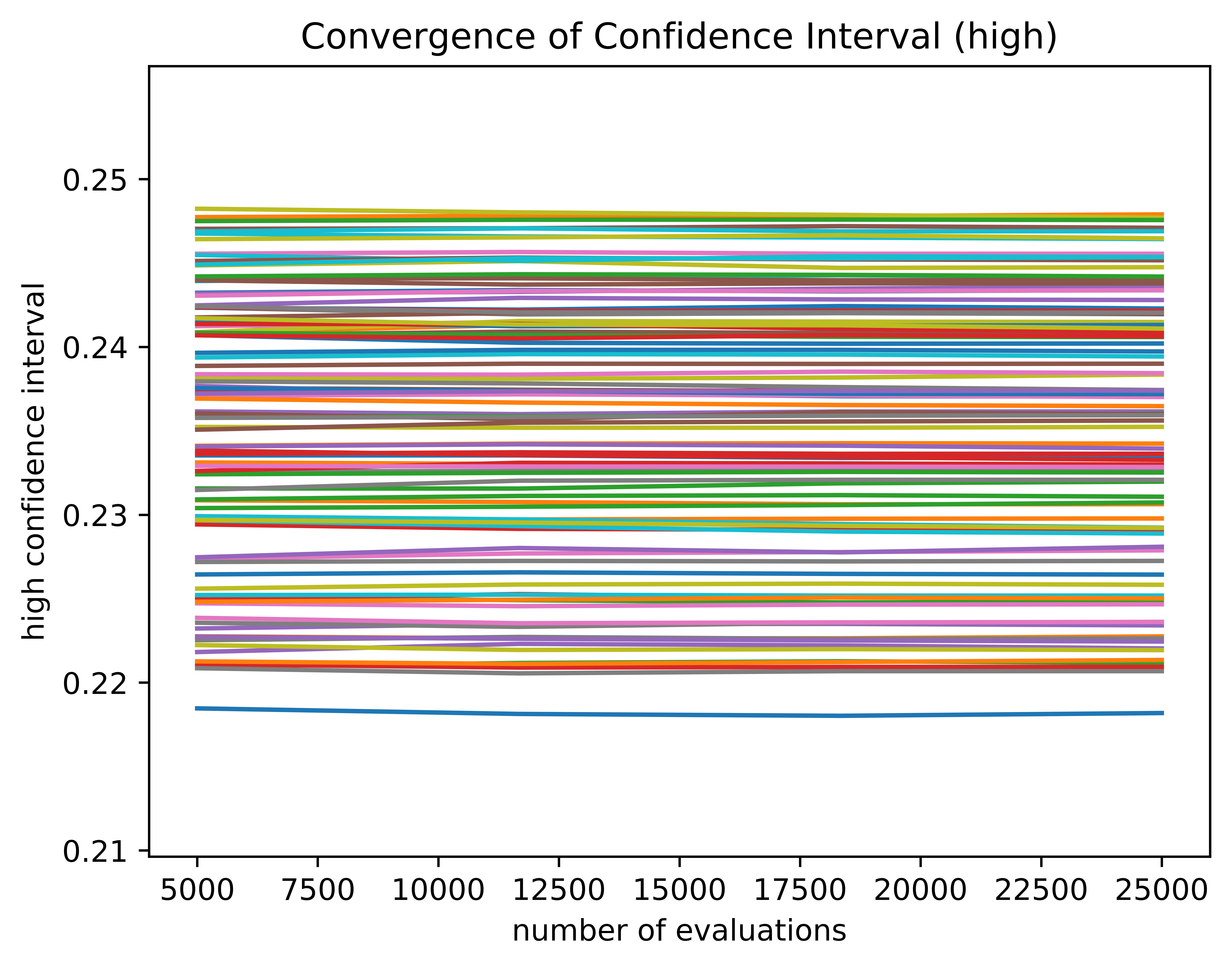
Fig. 17 The convergence of the upper intervals of the lift coefficient coefficient for each curve converging with additional evaluations.

Along with these convergence plots of the individual curves, the sets of curves have their overall convergence intervals written to a file.

The corresponding output of this file for the lift coefficient is shown below:

set: [0.18745724466451097, 0.24735395659860618]
set: [0.18607906409253214, 0.2475065011187474]
set: [0.18607906409253214, 0.2475065011187474]
set: [0.18607906409253214, 0.24759772917464634]

If the --verify flag is used with the included files, the user should get an output similar to the following for the lift coefficient:

Mean error between model and verification 3.146e-05

The user should get an output similar to the following for the drag coefficient:

Mean error between model and verification 1.3294e-06

Supersonic Diamond Airfoil

Background

The ground noise, obtained from the off-body pressure signature, is the response of interest in the case of the diamond airfoil. The inputs are the Mach number, the angle of attack (AoA), ground altitude, reflection factor (RF), x-velocity of wind, y-velocity of wind, relative humidity (hum), and temperature.

Outputs

When you run these files, you should get similar results to those below.

Table 3 UQPCE versus Monte Carlo mean, variance, and confidence intervals for the A-weighted decibels (dBA).

	UQPCE	Monte Carlo
mean	100.9	100.87
variance	0.098999	0.090497
confidence interval	[100.13, 101.72]	[100.31, 101.46]

If the --verify flag is used with the included files, the user should get an output similar to the following for the lift coefficient:

Mean error between model and verification 0.0086068

This value is similar to the mean error of the surrogate, 0.0061665, which suggests that the model is a good fit for the data.

Table 4 UQPCE versus Monte Carlo mean, variance, and confidence intervals for the C-weighted decibels (dBC).

	UQPCE	Monte Carlo
mean	116.5	116.48
variance	0.0781	0.0718
confidence interval	[115.92, 117.12]	[116.01, 116.97]

If the --verify flag is used with the included files, the user should get an output similar to the following for the lift coefficient:

Mean error between model and verification 0.0016291

This value is similar to the mean error of the surrogate, 0.0010945, which suggests that the model is a good fit for the data.

Table 5 UQPCE versus Monte Carlo mean, variance, and confidence intervals for the perceived loudness decibels (PLdB).

	UQPCE	Monte Carlo
mean	116.29	116.26
variance	0.1224	0.1124
confidence interval	[115.53, 117.17]	[115.46, 117.1]

The above chart shows the UQPCE versus Monte Carlo mean, variance, and confidence intervals for the perceived loudness (PLdB).

If the --verify flag is used with the included files, the user should get an output similar to the following for the lift coefficient:

Mean error between model and verification 0.012474

This value is similar to the mean error of the surrogate, 0.0079942, which suggests that the model is a good fit for the data.

OneraM6 Airfoil

Background

The lift coefficient (CL) and drag coefficient (CD) OneraM6 airfoil are studied. The inputs for the simulation are the Mach number and angle of attack.

Outputs

When you run these files, you should get results similar to those below.

Table 6 UQPCE versus Monte Carlo mean, variance, and confidence intervals for the lift coefficient.

	UQPCE	Monte Carlo
mean	0.29296	0.29288
variance	2.713e-4	2.739e-4
confidence interval	[0.26163, 0.3262]	[0.2611, 0.3259]

If the --verify flag is used, you will see output similar to below:

Mean error between model and verification 7.3086e-05

This value is similar to the mean error of the surrogate, 2.8925e-05, which suggests that the model is a good fit for the data.

Table 7 UQPCE versus Monte Carlo mean, variance, and confidence intervals for the drag coefficient.

	UQPCE	Monte Carlo
mean	0.01767	0.01766
variance	3.660e-06	3.686e-06
confidence interval	[0.0145, 0.0219]	[0.0144, 0.0219]

If the --verify flag is used, you will see output similar to below:

Mean error between model and verification 1.1883e-05

This value is similar to the mean error of the surrogate, 2.8941e-06, which suggests that the model is a good fit for the data.

The below plots are created using the --plot and --plot-stand flags. They represent the outputs for the drag coefficient case with order = 3.

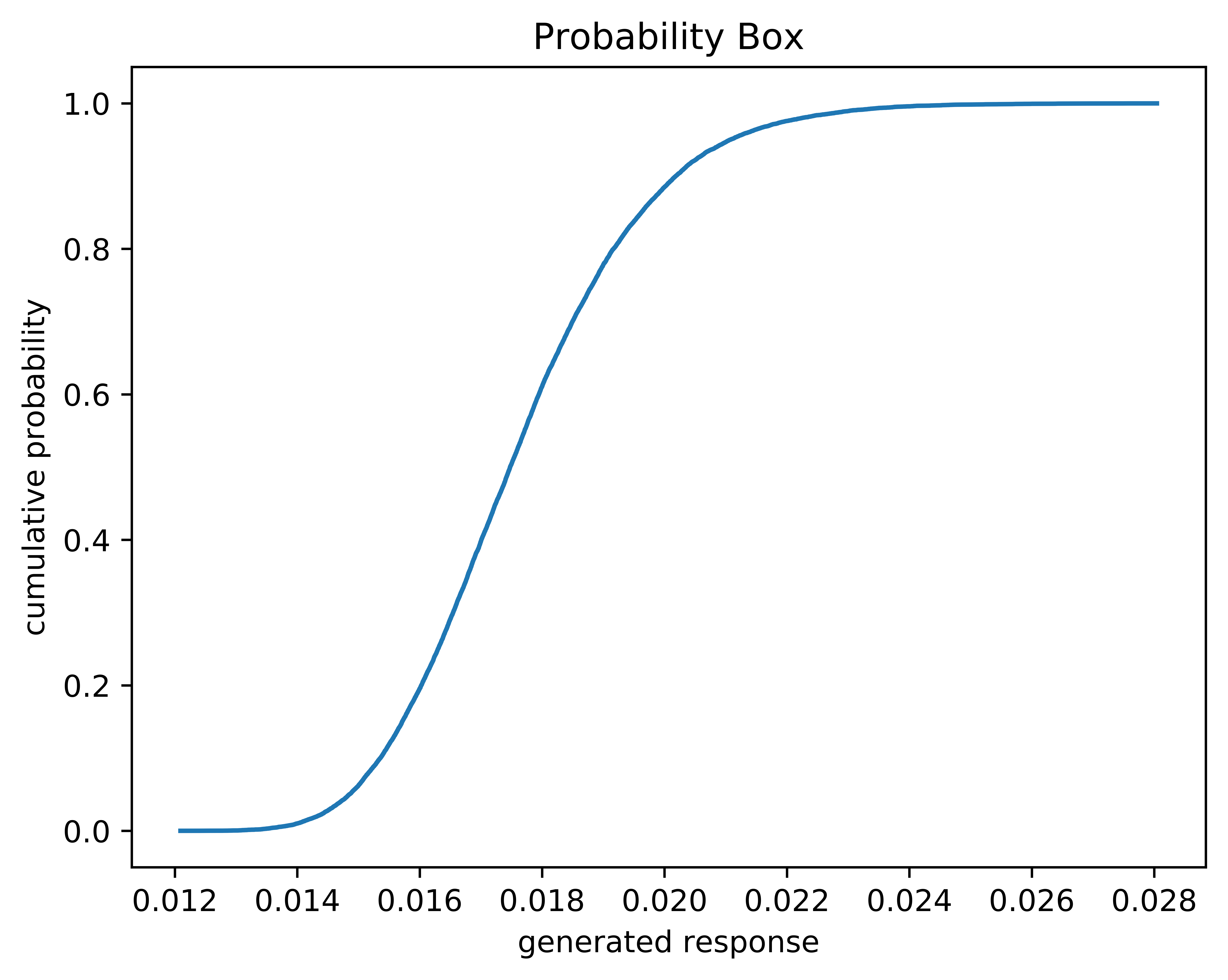
Fig. 18 The lift coefficient probability box for the OneraM6 airfoil.

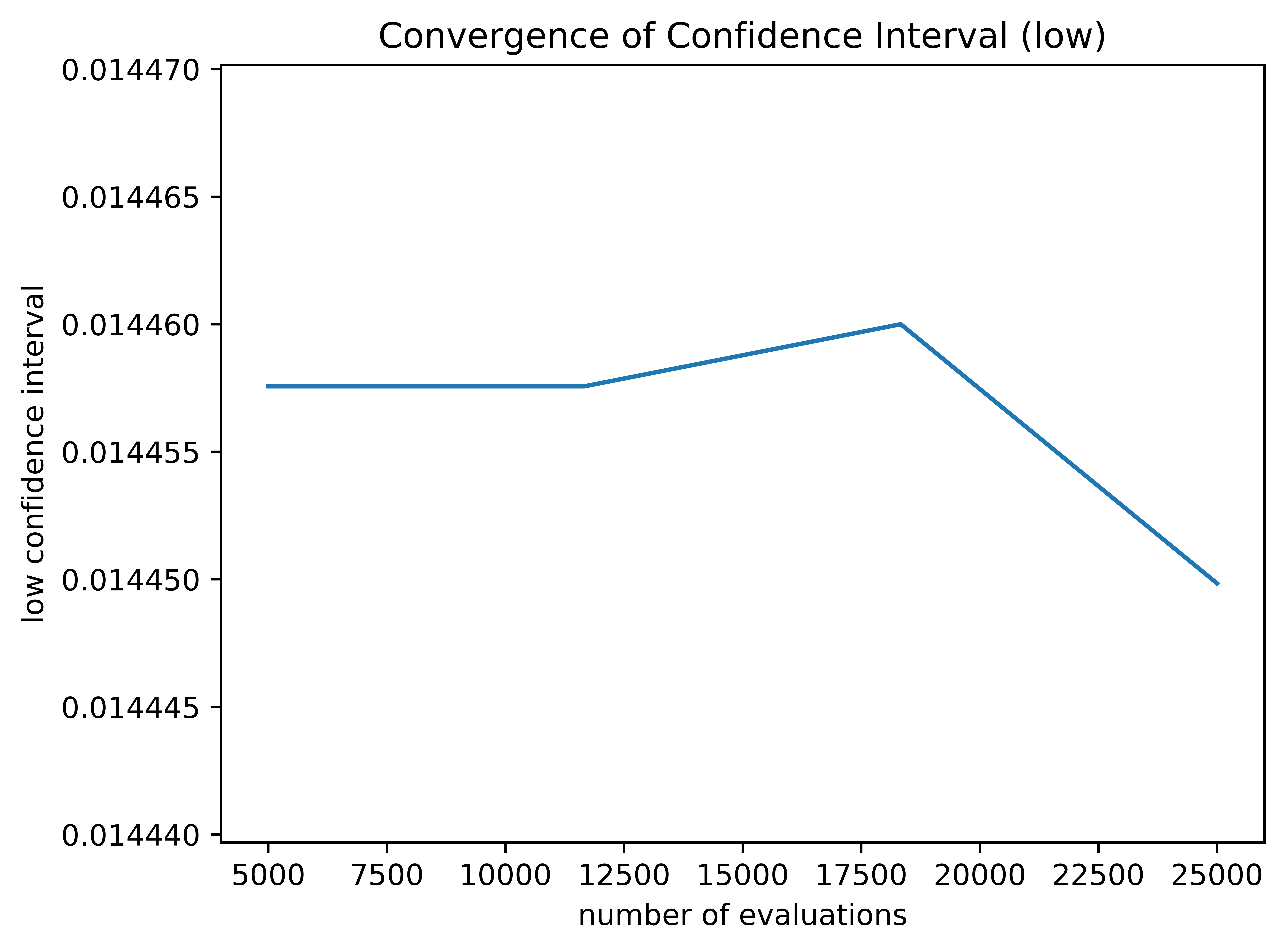
Fig. 19 The convergence of the lower confidence interval for the OneraM6 airfoil.

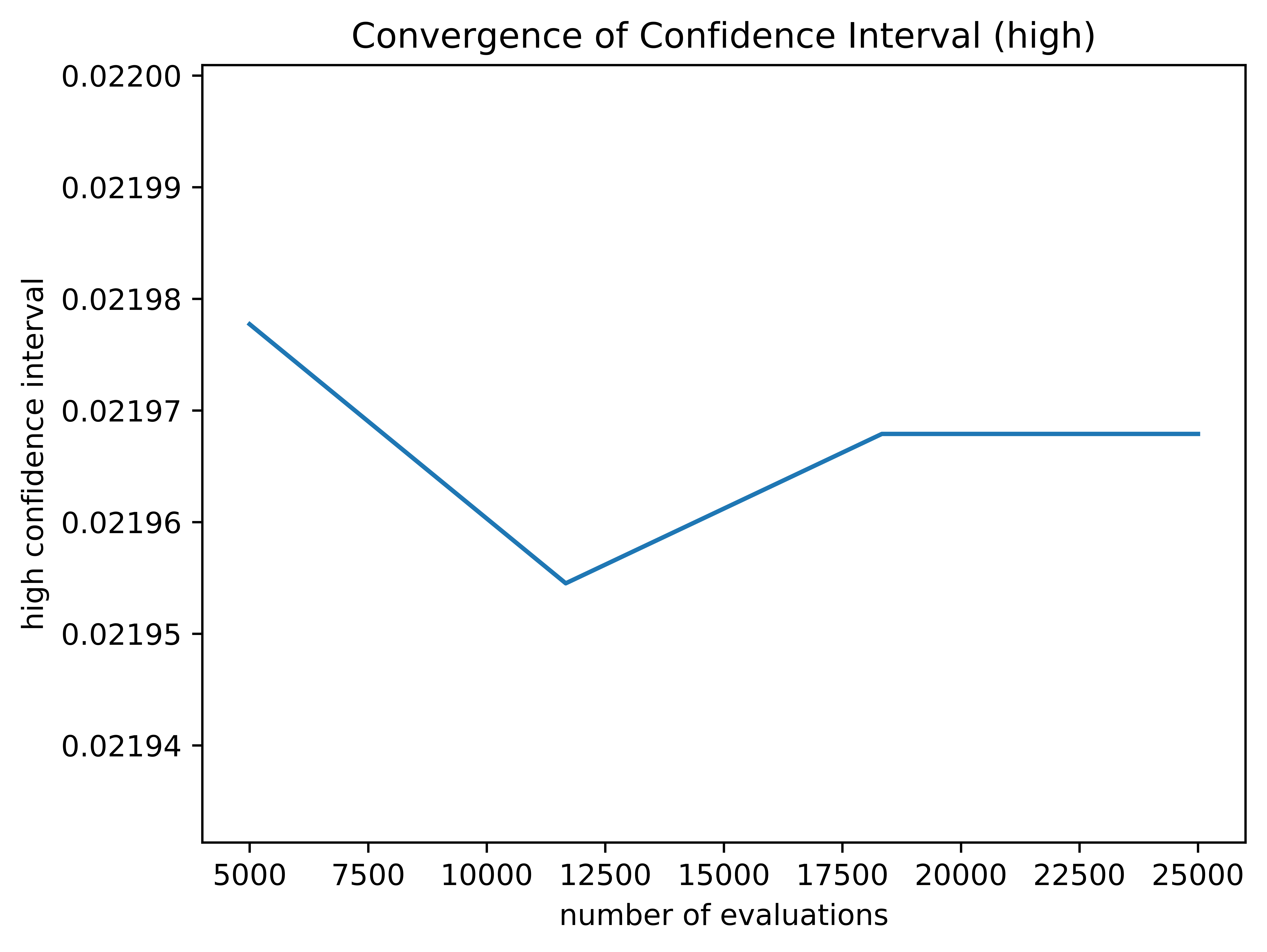
Fig. 20 The convergence of the upper confidence interval for the OneraM6 airfoil.

The file containing the convergence values looks like the following:

low:  [0.014457565322569664, 0.014457565322569664, 0.01445999863254389, 0.014449842360062486]
high: [0.021977720803637357, 0.02195451100712743, 0.021967892240129253, 0.021967892240129253]

The above figures show the probability box plot and the lower and upper confidence interval convergence for the OneraM6 airfoil case. Since none of the variables are epistemic, there is only one curve for the probability box. As shown, these confidence intervals did not converge within the accepted threshold and instead used the maximum number of samples allowed. It is possible for the curves to converge and not appear to be converged as long as the last two differences between confidence intervals are within the specified convergence threshold.

Analytical Case

Background

This case is included to demonstrate a case which uses all of the common variable types- normal, uniform, exponential, beta, and gamma. In addition to using all variable types, the values of the variables were generated using distributions from MATLAB, and an equation was used to generate the corresponding response. Since this example is completely analytical, we can solve for the exact Sobol values for comparison.

The equation used to generate the responses is given by

(22)\[ f(x_0,x_1,x_2,x_3,x_4) = x_0 + 2x_1 + 3x_2+ 4x_3 + x_4 + x_0x_1 + x_4^2 \]

Using properties of the variance operator below,

(23)\[ Var(aX) = a^2\sigma_{X}^2 \]

(24)\[ Var(X+Y) = \sigma_{X}^2 + \sigma_{Y}^2 + 2Cov(X,Y) \]

(25)\[ Var(XY) = (E(X^2Y^2)-E(XY)^2) \]

where \(Var\) is the variance, \(Cov\) is the covariance, and \(E\) is the expected value (mean), the expression for the variance of the function \(f\), is given by:

(26)\[ Var(f) = \sigma_{x_0}^2 + 4\sigma_{x_1}^2 + 9\sigma_{x_2}^2 + 16\sigma_{x_3}^2 + \sigma_{x_4}^2 + (E(x_0^2x_1^2)-E(x_0x_1)^2) + (E(x_4^2x_4^2)-E(x_4x_4)^2) + 2Cov(x_0+x_1,x_0x_1) + 2Cov(x_4x_4,x_4) \]

Variance for the distributions of the independent variables are given in table below.

Table 8 Distributions for independent variables in the analytical example case.

Distribution	Probability Density	Mean	Variance
normal	\(\frac{1}{\sqrt{2\pi\sigma^2}}e^{\frac{-(x-\mu)^2}{2\sigma^2}}\)	\(\mu\)	\(\sigma^2\)
uniform	\(\frac{1}{b-a}\)	\(\frac{1}{2}(a+b)\)	\(\frac{1}{12}(b-a)^2\)
exponential	\(\lambda e^{-\lambda x}\)	\(\frac{1}{\lambda}\)	\(\frac{1}{\lambda^2}\)
beta	\(\frac{x^{\alpha-1}(1-x)^{\beta-1}}{B(\alpha,\beta)}\)	\(\frac{\alpha}{\alpha+\beta}\)	\(\frac{\alpha\beta}{(\alpha+\beta)^2(\alpha+\beta+1)}\)
gamma	\(\frac{1}{\Gamma(\alpha)\theta^\alpha}x^{\alpha-1}e^{\frac{-x}{\theta}}\)	\(\alpha\theta\)	\(\alpha\theta^2\)

Evaluating the variances for each of the independent parameters gives \(Var(x_0)=0.25\), \(Var(x_1)=0.0208\), \(Var(x_2)=0.111\), \(Var(x_3)=0.0457\), \(Var(x_4)=0.25\). Substituting into Eq. (26) yields

(27)\[ Var(f) = 0.25 + 4(0.0208) + 9(0.111) + 16(0.0457) + 0.25 + 1.0257 + 1.2509 + 1.0825 + 0.9994 \]

Calculations for the covariance and expected quantity terms are left to the reader. Simplifying yields: \(Var(f) = 6.674\). To determine the total Sobol indices for this analytical function, the total variance is decomposed into individual variable contributions. For variables that do not have any interaction components, i.e. \(x_0x_1\), the decomposition is straight forward. The Sobol indices for \(x_2\), \(x_3\) and \(x_4\) are given below.

(28)\[ S_2 = \dfrac{ 9\sigma_{x_2}^2}{Var(f)} = 0.150 \]

(29)\[ S_3 = \dfrac{16\sigma_{x_3}^2}{Var(f)} = 0.110 \]

For \(x_4\) the total Sobol index includes the variance contributions from the quadratic terms as well.

(30)\[ S_4 = \dfrac{\sigma_{x_4}^2 + (E(x_4^2x_4^2)-E(x_4x_4)^2) + 2Cov(x_4x_4,x_4)}{Var(f)} = 0.374 \]

Sobol indices for \(x_0\) and \(x_1\) calculations are slightly more involved do to the interaction present. The variance contribution from the interaction term must be proportioned based on the ratio of the variable individual variances.

(31)\[ S_0 = \dfrac{ \sigma_{x_0}^2 + 4\sigma_{x_1}^2 + 2Cov(x_0+x_1,x_0x_1) + (E(x_0^2x_1^2)-E(x_0x_1)^2) }{Var(f)} \dfrac{\sigma_{x_0}}{\sigma_{x_0}+\sigma_{x_1}} = 0.338 \]

(32)\[ S_1 = \dfrac{ \sigma_{x_0}^2 + 4\sigma_{x_1}^2 + 2Cov(x_0+x_1,x_0x_1) + (E(x_0^2x_1^2)-E(x_0x_1)^2) }{Var(f)} \dfrac{\sigma_{x_1}}{\sigma_{x_0}+\sigma_{x_1}} = 0.028 \]

Outputs

Table 9 UQPCE versus Monte Carlo mean, variance, and confidence intervals for the analytical responses.

	UQPCE	Monte Carlo
mean	9.8	9.7989
variance	6.6741	6.6727
confidence interval	[5.6205, 15.5860]	[5.6365, 15.5405]

This shows similar results as above. This case has data that has no units and no physical meaning, and we still see that the results are similar between using UQPCE and Monte Carlo sampling the system.

Table 10 UQPCE versus Monte Carlo mean, variance, and confidence intervals for the analytical Sobols.

	UQPCE	Analytical Results
Sobol 0	0.3376	0.338
Sobol 1	0.0289	0.028
Sobol 2	0.1497	0.150
Sobol 3	0.1095	0.110
Sobol 4	0.3743	0.374

Verifying the Sobol sensitivities is not something that can be done to a system in which the underlying function is unknown. Since the underlying function is known in this case, the Sobol indices can be calculated.

If the --verify flag is used, you will see output similar to below:

Mean error between model and verification 2.3093e-14

This value is similar to the mean error of the surrogate, 2.6272e-14, which suggests that the model is a good fit for the data.

High Order Analytical Case

Background

This case is included to demonstrate a case using a high order response and PCE model. In addition to using all variable types, the values of the variables were generated using distributions from MATLAB, and an equation was used to generate the corresponding response. Since this example allows us to know the exact values for responses when Monte Carlo sampling the system, the correct Sobol values in addition to the mean and variance can be found.

The equation used to generate the responses is given by

(33)\[ f(x_0,x_1,x_2,x_3,x_4) = 0.02x_0 + 0.03x_0^4 + 0.08x_0^5 - 0.05x_1 - 0.02x_1^4 + x_1^5 + x_2 + x_2^4 - 100x_2^5 - x_3 - x_3^4 + 1000x_3^5 - 0.09x_4 - 0.01x_4^4 + 0.01x_4^5 \]

Outputs

Table 11 UQPCE versus Monte Carlo mean, variance, and confidence intervals for the high order analytical responses.

	UQPCE	Monte Carlo
mean	11.409	11.403
variance	418.27	421.18
confidence interval	[0.2492, 40.507]	[0.2542, 40.205]

This shows similar results as above. This case has data that has no units and no physical meaning, and we still see that the results are similar between using UQPCE and Monte Carlo sampling the system.

Table 12 UQPCE versus Monte Carlo Sobols for the high order analytical responses.

	UQPCE	Monte Carlo
Sobol 0	0.0399	0.0404
Sobol 1	0.1504	0.1530
Sobol 2	0.2993	0.3008
Sobol 3	0.3094	0.3135
Sobol 4	0.2011	0.1926

Verifying the Sobol sensitivities is not something that can be done to a system in which the underlying function is unknown. Since the underlying function is known in this case, the Sobol indices can be calculated.

If the --verify flag is used, you will see output similar to below:

Mean error between model and verification 2.7579e-09

This value is similar to the mean error of the surrogate, 2.9757e-09, which suggests that the model is a good fit for the data.

User Input Variable Case

Background

This case is included to demonstrate the accuracy and flexibility of inputting variables according to their equation instead of variable type.

Note

Using the equation approach for inputting a variable of one of the variable types (normal, uniform, beta, exponential, and gamma) is not recommended when running the program. It will give you equivalent outputs, but the equation-based approach is much slower than the using the variable types.

The equation used to generate the responses is given by Eq. (22).

Outputs

Table 13 UQPCE versus Monte Carlo mean, variance, and confidence intervals for the user-input variable example.

	UQPCE	Monte Carlo
mean	17.645	17.643
variance	15.225	15.219
confidence interval	[10.591, 25.657]	[10.731, 25.864]

Table 14 UQPCE versus Monte Carlo Sobols for the user-input variable example.

	UQPCE	Monte Carlo
Sobol 0	0.1199	0.1198
Sobol 1	0.3230	0.3231
Sobol 2	0.0328	0.0329
Sobol 3	0.4912	0.4912
Sobol 4	0.0422	0.0422

If the --verify flag is used, you will see output similar to below:

Mean error between model and verification 4.2751e-14

This value is similar to the mean error of the surrogate, 2.8777e-14, which suggests that the model is a good fit for the data.

Interval Case

Background

This case is included to demonstrate the accuracy of modeling distributions with non-standard bounds on variables.

The equation used to generate the responses is given by

\[ f(x_0,x_1,x_2,x_3,x_4,x_5) = x_0 + 2 x_1 + 3 x_2+ 4 x_3 + x_4 + x_0 x_1 + x_4^2 + 3 x_5 x_2 \]

Outputs

Table 15 UQPCE versus Monte Carlo mean, variance, and confidence intervals for the interval variable example.

	UQPCE	Monte Carlo
mean	123.6	123.60
variance	2567.5	2566.85
confidence interval	[54.931, 249.540]	[54.267, 248.388]

Table 16 UQPCE versus Monte Carlo Sobols for the interval variable example.

	UQPCE	Monte Carlo
Sobol 0	0.0034	0.0035
Sobol 1	0.0042	0.0042
Sobol 2	0.1995	0.1994
Sobol 3	0.0011	0.0011
Sobol 4	0.0025	0.0026
Sobol 5	0.8113	0.8113

If the --verify flag is used, you will see output similar to below:

Mean error between model and verification 0.014425

This value is similar to the mean error of the surrogate, 0.0044884, which suggests that the model is a good fit for the data.

Small Mean Case

Background

This case is included to demonstrate the accuracy of a case with a small mean.

The equation used to generate the responses is given by

\[ f(x_0,x_1,x_2,x_3,x_4,x_5) = 0.0000001(0.05x_0 + x_1^2 - 1.5x_3^2 + x_2 + x_1 + 0.1x_4x_5) \]

Outputs

Table 17 UQPCE versus Monte Carlo mean, variance, and confidence intervals for the small mean example.

	UQPCE	Monte Carlo
mean	6.4413e-7	6.4412e-07
variance	1.6863e-14	1.6860e-14
confidence interval	[4.073e-7, 9.137e-7]	[4.060e-07, 9.140e-07]

Table 18 UQPCE versus Monte Carlo Sobols for the small mean example.

	UQPCE	Monte Carlo
Sobol 0	0.0237	0.0237
Sobol 1	0.2123	0.2124
Sobol 2	0.3012	0.3011
Sobol 3	0.1647	0.1648
Sobol 4	0.1379	0.1377
Sobol 5	0.1779	0.1780

If the --verify flag is used, you will see output similar to below:

Mean error between model and verification 5.1457e-22

This value is similar to the mean error of the surrogate, 3.7852e-22, which suggests that the model is a good fit for the data.

Discrete Case

Background

This case is included to demonstrate the use of the discrete variables.

The equation used to generate the responses is given by

\[ f(x_0,x_1,x_2,x_3,x_4,x_5,x_6,x_7) = x_0^2 + 3x_1^2 + 20x_2^2 + 50x_3^3 + x_0 + 0.3x_4 + (0.15x_4)^2 + 0.07x_5^3 - x_6^2 - 0.004x_7 + 0.03x_7^3 \]

Outputs

Table 19 UQPCE versus Monte Carlo mean, variance, and confidence intervals for the discrete variable example.

	UQPCE	Monte Carlo
mean	47.366	47.366
variance	190.33	190.37
confidence interval	[24.44, 76.76]	[24.37, 76.48]

Table 20 UQPCE versus Monte Carlo Sobols for the discrete variable example.

	UQPCE	Monte Carlo
Sobol 0	0.0213	0.0213
Sobol 1	0.0673	0.0672
Sobol 2	0.0175	0.0175
Sobol 3	0.0113	0.0113
Sobol 4	0.0170	0.0170
Sobol 5	0.1449	0.1449
Sobol 6	0.0941	0.0938
Sobol 7	0.6266	0.6266

If the --verify flag is used, you will see output similar to below:

Mean error between model and verification 1.1622e-12

This value is similar to the mean error of the surrogate, 1.1623e-12, which suggests that the model is a good fit for the data.

Discrete Parabola Case

Background

This case is included to demonstrate the use of the discrete variables.

The equation used to generate the responses is given by

\[ f(x_0,x_1,x_2,x_3) = \frac{1}{3}(15 + 3x_0 + 4x_0^2) + \frac{1}{3}(16 + 2x_1 + x_1^2) - \frac{1}{3}(5 + 0.8x_2 + 0.03x_2^2) + \frac{1}{3}(4 - x_3 + 4x_3^2) \]

Variances for the distributions of the variables are given in table below.

Using the mean of each variable to hold the variables constant, the Sobols are calculated using one-variable-at-a-time variable decomposition. The means of the independent variables are given in the above table.

Outputs

Table 21 UQPCE versus Monte Carlo mean, variance, and confidence intervals for the discrete parabola example.

	UQPCE	Monte Carlo
mean	12.416	12.416
variance	48.815	48.824
confidence interval	[-0.027, 27.79]	[-0.04, 27.84]

Table 22 UQPCE versus Monte Carlo Sobols for the discrete parabola example.

	UQPCE	Monte Carlo
Sobol 0	0.2887	0.2888
Sobol 1	0.1554	0.1553
Sobol 2	0.2724	0.2722
Sobol 3	0.2836	0.2835

If the --verify flag is used, you will see output similar to below:

Mean error between model and verification 5.4386e-14

This value is similar to the mean error of the surrogate, 3.0609e-14, which suggests that the model is a good fit for the data.

User Input Continuous and Discrete Case

Background

This case is included to demonstrate the use of both continuous and discrete user input variables in the same case.

The equation used to generate the responses is given by

\[ f(x_0,x_1,x_2,x_3,x_4,x_6,x_7) = \]

Outputs

Table 23 UQPCE versus Monte Carlo mean, variance, and confidence intervals for the user-input continuous and discrete variable example.

	UQPCE	Monte Carlo
mean	9.4994	9.4995
variance	3.8326	3.8332
confidence interval	[5.739, 13.505]	[5.683, 13.490]

Table 24 UQPCE versus Monte Carlo Sobols for the user-input continuous and discrete variable example.

	UQPCE	Monte Carlo
Sobol 0	0.1099	0.1100
Sobol 1	0.0870	0.0868
Sobol 2	0.0235	0.0235
Sobol 3	0.1220	0.1219
Sobol 4	0.2854	0.2855
Sobol 5	0.2348	0.2348
Sobol 6	0.0905	0.0904
Sobol 7	0.0469	0.0470

If the --verify flag is used, you will see output similar to below:

Mean error between model and verification 2.5882e-13

This value is similar to the mean error of the surrogate, 2.7263e-13, which suggests that the model is a good fit for the data.