Confidence Interval#
To demonstrate the validity of the technique used to calculate the confidence interval, several known distributions will have their known analytical confidence interval compared to the result from our method.
Continuous Cases#
In this section, we will demonstrate the technique on all of the continuous distributions that UQPCE supports.
Uniform Distribution#
The analytical bound is 8.95
The interpolated bound is 8.950277749906654
The solved bound is 8.95013551407136
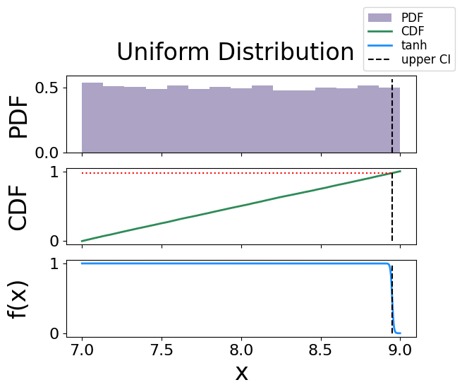
Fig. 21 The figure of solving for the confidence interval using the activation function technique for a uniform distribution.#
Normal Distribution#
The analytical bound is 0.9199279690801081
The interpolated bound is 0.8872625602584633
The solved bound is 0.8863382411126177
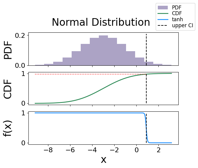
Fig. 22 The figure of solving for the confidence interval using the activation function technique for a normal distribution.#
Beta Distribution#
The analytical bound is 0.9999999999999958
The interpolated bound is 0.9999999999999958
The solved bound is 0.9999999999997697
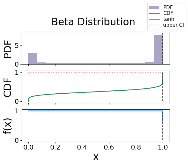
Fig. 23 The figure of solving for the lower confidence bound using the activation function technique for a beta distribution.#
Exponential Distribution#
The analytical bound is 0.008439269328096625
The interpolated bound is 0.008518509775512847
The solved bound is 0.008525717739948167
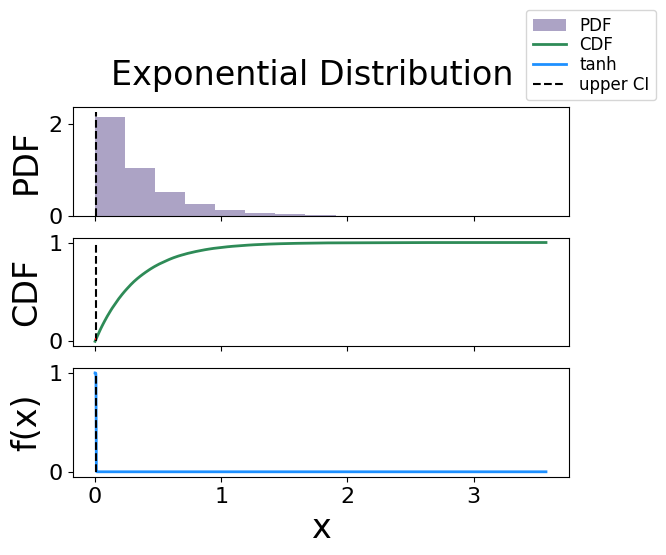
Fig. 24 The figure of solving for the lower confidence bound using the activation function technique for a exponential distribution.#
The analytical bound is 1.229626484704645
The interpolated bound is 1.2318518105534306
The solved bound is 1.2320707235826833
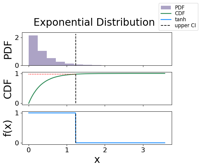
Fig. 25 The figure of solving for the upper confidence bound using the activation function technique for a exponential distribution.#
Gamma Distribution#
The analytical bound is -0.9394476803640087
The interpolated bound is -0.9376203388918325
The solved bound is -0.9376873865022382
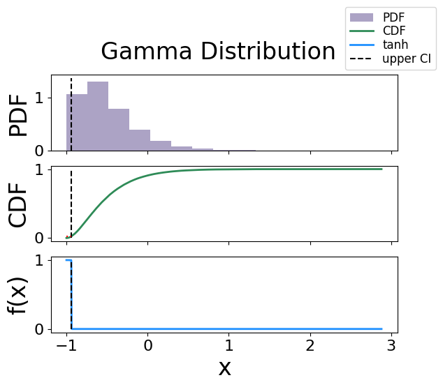
Fig. 26 The figure of solving for the confidence interval using the activation function technique for a gamma distribution.#
Discrete Cases#
In this section, we will demonstrate the technique on all of the discrete distributions that UQPCE supports.
Poisson Distribution#
The analytical bound is 2.0
The interpolated bound is 2.0
The solved bound is 2.000000000001842
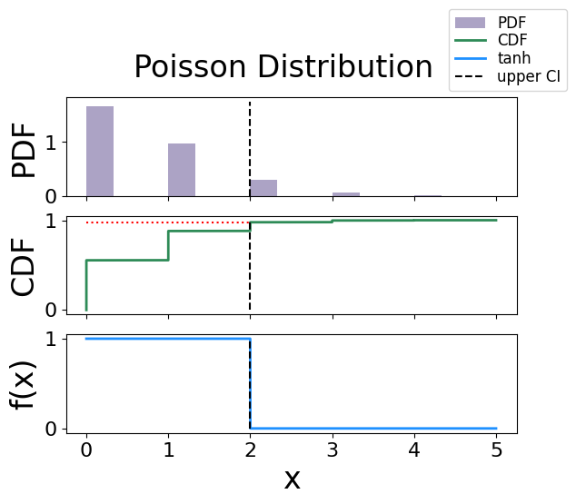
Fig. 27 The figure of solving for the confidence interval using the activation function technique for a Poisson distribution.#
Negative Binomial Distribution#
The analytical bound is 12.0
The interpolated bound is 12.0
The solved bound is 12.000000000002276
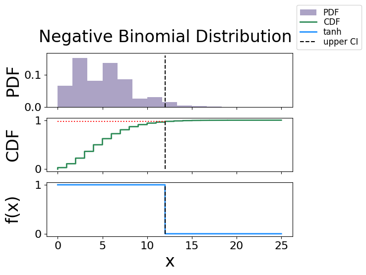
Fig. 28 The figure of solving for the confidence interval using the activation function technique for a negative binomial distribution.#
Hypergeometric Distribution#
The analytical bound is 6.0
The interpolated bound is 6.0
The solved bound is 6.00000000000082
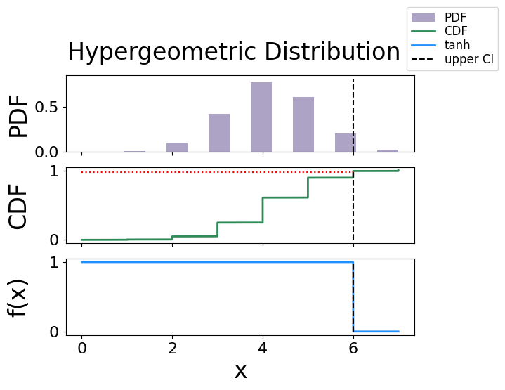
Fig. 29 The figure of solving for the confidence interval using the activation function technique for a hypergeometric distribution.#
Uniform Distribution#
The analytical bound is 8.0
The interpolated bound is 8.0
The solved bound is 8.00000000000125
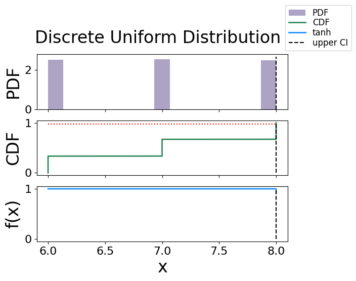
Fig. 30 The figure of solving for the confidence interval using the activation function technique for a discrete uniform distribution.#
Epistemic Cases#
In this section, we will demonstrate the technique on an epistemic case with multiple aleatory curves.