# !pip install "ray[default]"3 Equivalent Water Thickness/Canopy Water Content from Imaging Spectroscopy Data
This notebook is part of a numbered series (01-05) that focuses specifically on using EMIT and ECOSTRESS Data together to prepare for future SBG research.
Summary
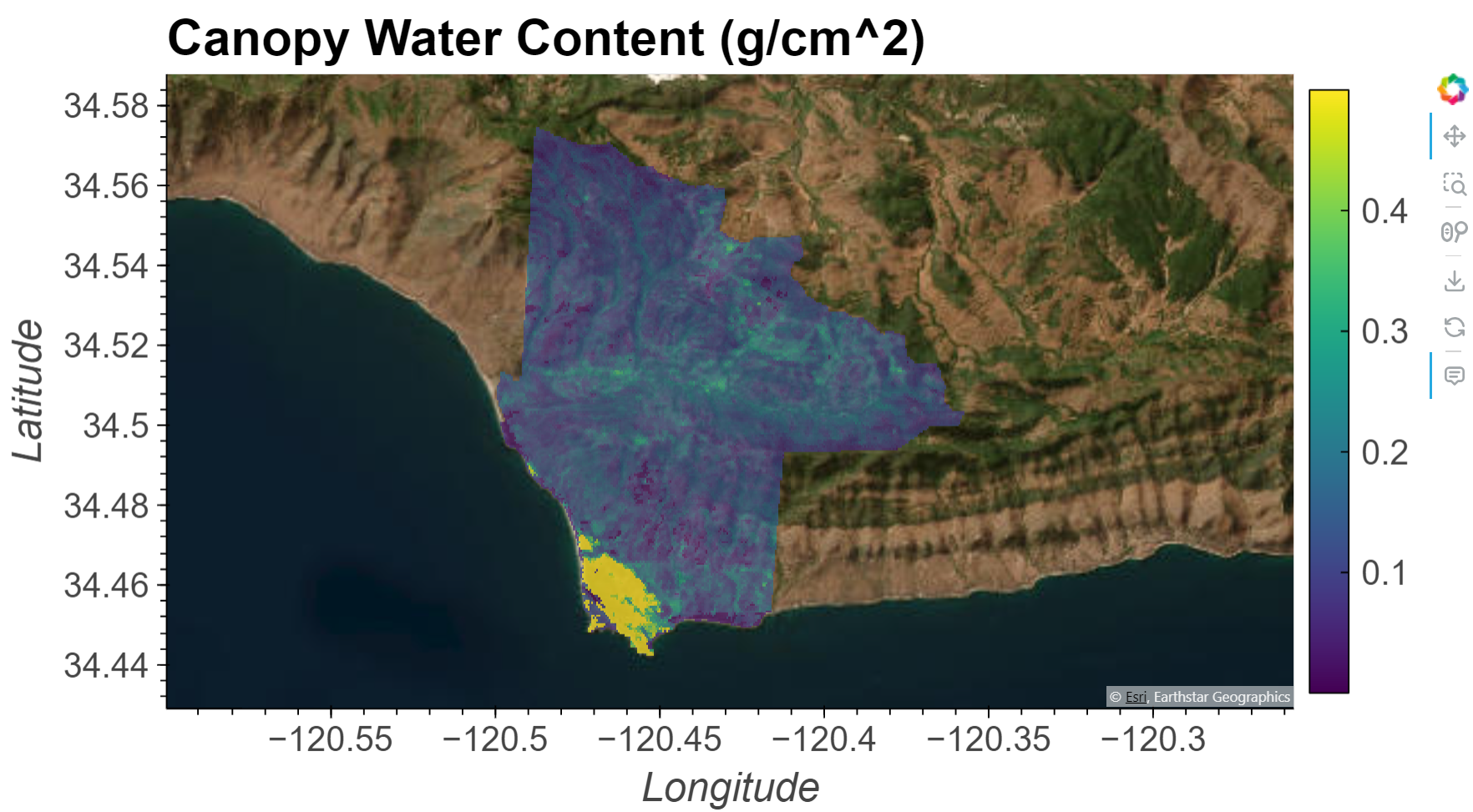
In this notebook we will explore how Equivalent Water Thickness (EWT) or Canopy Water Content (CWC) can be calculated from the Earth Surface Mineral Dust Source Investigation (EMIT) L2A Reflectance Product, then we will apply this knowledge to calculate CWC over the Jack and Laura Dangermond Preserve located near Santa Barbara, CA.
Background
Equivalent Water Thickness (EWT) is the predicted thickness or absorption path length in centimeters (cm) of water that would be required to yield an observed spectra. In the context of vegetation, this is equivalent to canopy water content (CWC) in g/cm^2 because a cm^3 of water has a mass of 1g.
CWC can be derived from surface reflectance spectra because they provide information about the composition of the target, including water content. Reflectance is the fraction of incoming solar radiation reflected by Earth’s surface. Different materials reflect varying proportions of radiation based upon their chemical composition and physical properties, giving materials their own unique spectral signature or fingerprint. In particular, liquid water causes characteristic absorption features to appear in the near-infrared wavelengths of the solar spectrum, which enables an estimation of its content.
CWC correlates with vegetation type and health, as well as wildfire risk. The methods used here to calculate CWC are based on the ISOFIT python package. The Beer-Lambert physical model used to calculate CWC is described in Green et al. (2006) and Bohn et al. (2020). It uses wavelength-dependent absorption coefficients of liquid water to determine the absorption path length as a function of absorption feature depth. Of note, this model does not account for multiple scattering effects within the canopy and may result in overestimation of CWC (Bohn et al., 2020).
The Jack and Laura Dangermond Preserve and its surrounding lands are one of the last “wild coastal” regions in Southern California. The preserve is over 24,000 acres and consists of several ecosystem types and is home to over 600 plant species and over 200 wildlife species.
More about the EMIT mission and EMIT products.
References
- Shrestha, Rupesh. 2023. Equivalent water thickness/canopy water content from hyperspectral data. Jupyter Notebook. Oak Ridge National Laboratory Distributed Active Archive Center. https://github.com/rupesh2/ewt_cwc/tree/main
- Bohn, N., L. Guanter, T. Kuester, R. Preusker, and K. Segl. 2020. Coupled retrieval of the three phases of water from spaceborne imaging spectroscopy measurements. Remote Sensing of Environment 242:111708. https://doi.org/10.1016/j.rse.2020.111708
- Green, R.O., T.H. Painter, D.A. Roberts, and J. Dozier. 2006. Measuring the expressed abundance of the three phases of water with an imaging spectrometer over melting snow. Water Resources Research 42:W10402. https://doi.org/10.1029/2005WR004509
- Thompson, D.R., V. Natraj, R.O. Green, M.C. Helmlinger, B.-C. Gao, and M.L. Eastwood. 2018. Optimal estimation for imaging spectrometer atmospheric correction. Remote Sensing of Environment 216:355–373. https://doi.org/10.1016/j.rse.2018.07.003
Requirements - NASA Earthdata Account
- No Python setup requirements if connected to the workshop cloud instance!
- Local Only Set up Python Environment - See setup_instructions.md in the /setup/ folder to set up a local compatible Python environment
- Downloaded necessary files. This is done at the end of the 01_Finding_Concurrent_Data notebook.
Learning Objectives
- Calculate CWC of a single pixel
- Calculate CWC of an ROI
Tutorial Outline
3.1 Setup
3.2 Opening EMIT Data
3.3 Extracting Reflectance of a Pixel
3.4 Calculating CWC
3.4.1 Single Point
3.4.2 DataFrame of Points
3.5 Applying Inversion in Parallel Across an ROI
3.1 Setup
Uncomment the below cell and install the ray python library. This is only necessary if using the 2i2c Cloud Instance.
Import the required libraries.
# Import Packages
import os
# Some cells may generate warnings that we can ignore. Comment below lines to see.
import warnings
warnings.filterwarnings('ignore')
import numpy as np
import xarray as xr
from osgeo import gdal
import rasterio as rio
import rioxarray as rxr
from matplotlib import pyplot as plt
import hvplot.xarray
import hvplot.pandas
import pandas as pd
import earthaccess
from modules.emit_tools import emit_xarray
from modules.ewt_calc import calc_ewt
from scipy.optimize import least_squares3.2 Open an EMIT File
EMIT L2A Reflectance Data are distributed in a non-orthocorrected spatially raw NetCDF4 (.nc) format consisting of the data and its associated metadata. To work with this data, we will use the emit_xarray function from the emit_tools.py module included in the repository.
3.2.1 Streaming Data
As we did in the previous notebook, to stream the data, log in using earthaccess, then start and https session and open the url for the scene.
# Login to NASA Earthdata
earthaccess.login(persist=True)
# Get Https Session using Earthdata Login Info
fs = earthaccess.get_fsspec_https_session()
# Define Local Filepath
fp = fs.open('https://data.lpdaac.earthdatacloud.nasa.gov/lp-prod-protected/EMITL2ARFL.001/EMIT_L2A_RFL_001_20230401T203751_2309114_002/EMIT_L2A_RFL_001_20230401T203751_2309114_002.nc')3.2.2 Downloading Data
If you have downloaded the data, you can just set the filepath.
# fp = '../data/EMIT_L2A_RFL_001_20230401T203751_2309114_002.nc'Open the file using the emit_xarray function.
ds = emit_xarray(fp,ortho=True).load()Set the fill values equal to np.nan improved visualization.
ds.reflectance.data[ds.reflectance.data == -9999] = np.nanSimilarly to what we did in the previous notebook, we can plot a single band to get an idea of where our scene is. This is the same scene we processed earlier.
emit_layer = ds.sel(wavelengths=850,method='nearest')
emit_layer.hvplot.image(cmap='viridis',geo=True, tiles='ESRI', frame_width=720,frame_height=405, alpha=0.7, fontscale=2).opts(
title=f"{emit_layer.wavelengths:.3f} {emit_layer.wavelengths.units}", xlabel='Longitude',ylabel='Latitude')