
Modeling and Sim Guide#
The Prognostics Python Package (ProgPy) includes tools for defining, building, using, and testing models for prognostics of engineering systems. It also provides a set of prognostics models for select components developed within this framework, suitable for use in prognostics applications for these components and can be used in conjunction with the state estimation and prediction features (see State Estimation and Prediction Guide) to perform research in prognostics methods.
Installing ProgPy#
The latest stable release of ProgPy is hosted on PyPi. For most users, this version will be adequate. To install via the command line, use the following command:
$ pip install progpy
If you will be using the datadriven tools (e.g., LSTM model), install the datadriven dependencies as well using the following command:
$ pip install 'progpy[datadriven]'
Users who would like to contribute to ProgPy or would like to use pre-release features can do so using the ProgPy GitHub repo. This isn’t recommended for most users as this version may be unstable. To do this, use the following commands:
$ git clone https://github.com/nasa/progpy
$ cd progpy
$ git checkout dev
$ pip install -e .
If you will be using the datadriven tools (e.g., LSTM model), install the datadriven dependencies as well using the following command:
$ pip install -e '.[datadriven]'
For help with troubleshooting, see the Troubleshooting Guide.
Getting Started#
The best way to learn how to use progpy is through the tutorial. There are also a number of examples that show different aspects of the package, summarized and linked in the below sections
ProgPy Prognostic Model Format#
Prognostics models are the foundation of the prognostics process. They describe how a system or system-of-systems is expected to behave based on how it is used/loaded (i.e., input). Prognostic models typically come in one of 4 categories: knowledge-based, physics-based, data-driven, or some combination of those three (i.e., hybrid).
Inputs#
Prognostic model inputs are how a system is loaded. These are things that can be controlled, and affect how the system state evolves. The expected inputs for a model are defined by its inputs property. For example, a battery is loaded by applying a current, so the only input is i, the applied current. Inputs are also sometimes environmental conditions, such as ambient temperature or pressure.
Inputs are one of the inputs to the state transition model, described in States .
States#
ProgPy prognostic models are state-transition models. The internal state of the system at any time is represented by one or more (frequently hidden) state variables, represented by the custom type StateContainer. Each model has a discrete set of states, the keys of which are defined by the states property.
For example, the example ThrownObject model has two states, position (x) and velocity (v).
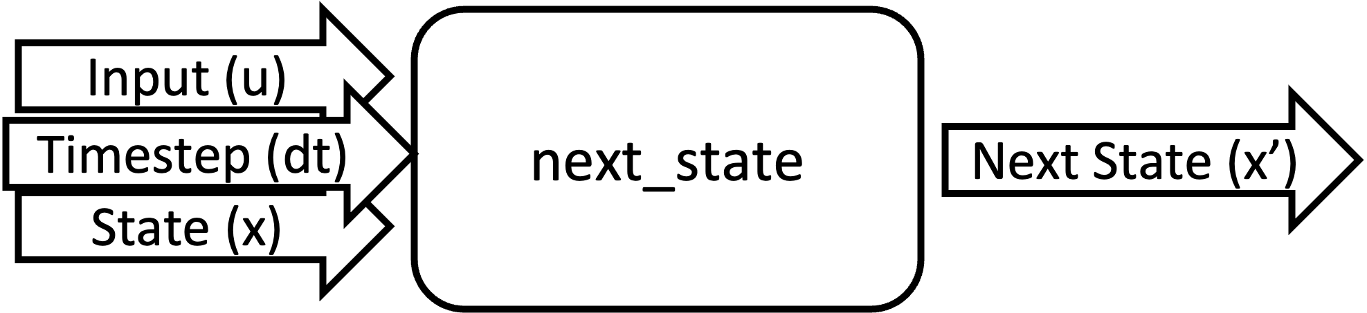
States are transitioned forward in time using the state transition equation.
\(x(t+dt) = f(t, x(t), u(t), dt, \Theta)\)
where \(x(t)\) is state at time \(t\), \(u(t)\) is input at time \(t\) , \(dt\) is the stepsize, and \(\Theta\) are the model parameters .
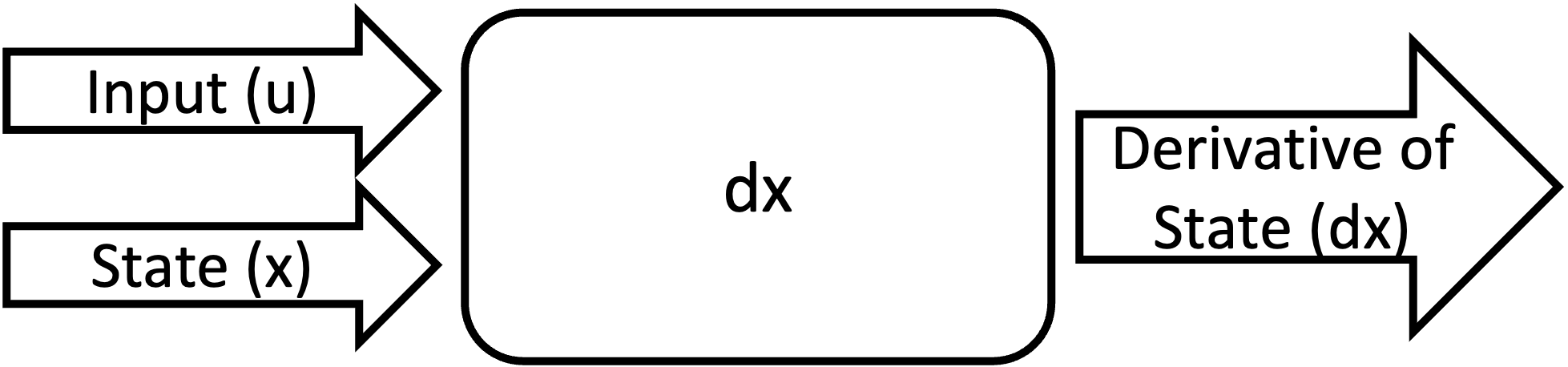
In a ProgPy model, this state transition can be represented one of two ways, either discrete or continuous, depending on the nature of state transition. In the case of continuous models, state transition behavior is defined by defining the first derivative, using the progpy.PrognosticsModel.dx() method. For discrete models, state transition behavior is defined using the progpy.PrognosticsModel.next_state() method. The continuous state transition behavior is recommended, because defining the first derivative enables some approaches that rely on that information.
States can also be discrete or continuous. Discrete states are those which can only exist in a finite set of values. Continuous states are initialized with a number and discrete states are initialized using the function progpy.create_discrete_state(), like the examples below. Each discrete state represents a unique condition or mode, and transitions between states are governed by defined rules or events, providing clarity and predictability in state management.
>>> from progpy import create_discrete_state
>>> ValveState = create_discrete_state(2, ["open", "closed"])
>>> x["valve"] = ValveState.open
>>> from progpy import create_discrete_state
>>> GearState = create_discrete_state(5, transition="sequential")
>>> x["gear"] = GearState(1)
Note
Discrete states are different from discrete models. Discrete models are models where state transition is discrete, where discrete states are where the state itself is discrete. Discrete models may have continuous states.
State Transition Equation Example
An example of a state transition equation for a thrown object is included below. In this example, a model is created to describe an object thrown directly into the air. It has two states: position (x) and velocity (v), and no inputs.
>>> def dx(self, x, u):
>>>    # Continuous form
>>>    dxdt = x['v']
>>>    dvdt = -9.81  # Acceleration due to gravity
>>>    return self.StateContainer({'x': dxdt, 'v': dvdt})
or, alternatively
>>> def next_state(self, x, u, dt):
>>>    # Discrete form
>>>    new_x = x['x'] + x['v']*dt
>>>    new_v = x['v'] -9.81*dt  # Acceleration due to gravity
>>>    return self.StateContainer({'x': new_x, 'v': new_v})
Output (Measurements)#
The next important part of a prognostic model is the outputs. Outputs are measurable quantities of a system that are a function of system state. When applied in prognostics, generally the outputs are what is being measured or observed in some way. State estimators use the different between predicted and measured values of these outputs to estimate the system state.
Outputs are a function of only the system state (x) and parameters (\(\Theta\)), as described below. The expected outputs for a model are defined by its outputs property. The logic of calculating outputs from system state is provided by the user in the model progpy.PrognosticsModel.output() method.
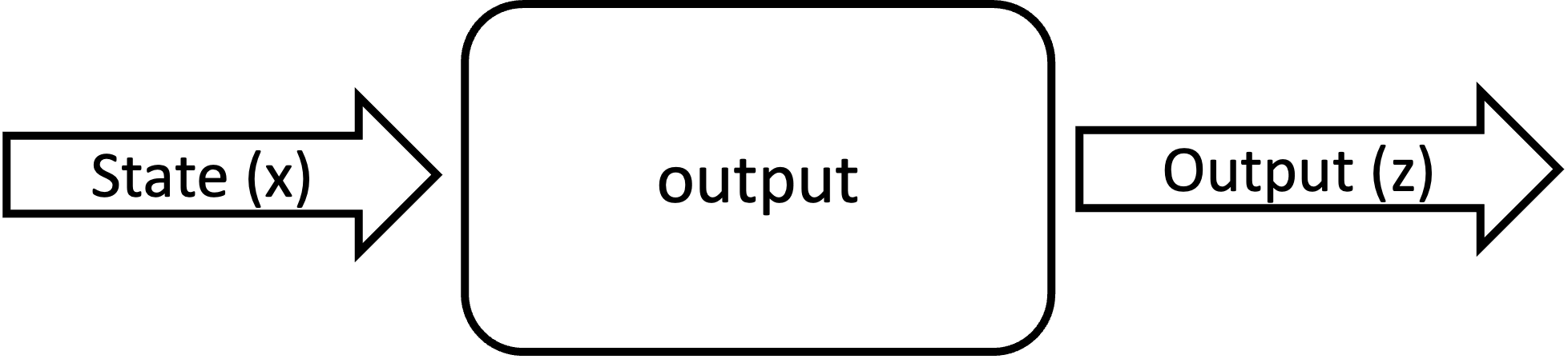
\(z(t) = f(x(t), \Theta)\)
Output Equation Example
An example of a output equation for a thrown object is included below. In this example, a model is created to describe an object thrown directly into the air. It has two states: position (x) and velocity (v). In this case we’re saying that the position of the object is directly measurable.
>>> def output(self, x):
>>>     # Position is directly measurable
>>>     position = x['x']
>>>     return self.OutputContainer({'x': position})
Events#
Traditionally users may have heard the prognostic problem as estimating the Remaining Useful Life (RUL) of a system. ProgPy generalizes this concept with the concept of events. ProgPy Prognostic Models contain one or more events which can be predicted. Systems frequently have more than one failure mode, each of these modes can be represented by a separate event. For example, a valve model might have separate events for an internal leak and a leak at the input. Or a battery model might have events for insufficient capacity, thermal runaway, and low-voltage.
Additionally, events can be used to predict other events of interest beyond failure, such as special system states or warning thresholds. For example, the above battery model might also have an warning event for when battery capacity reaches 50% of the original capacity because of battery aging with use.
The expected events for a model are defined by its events property. The logic of events can be defined in two methods: progpy.PrognosticsModel.threshold_met() and progpy.PrognosticsModel.event_state().
Thresholds are the conditions under which an event occurs. The logic of the threshold is defined in the progpy.PrognosticsModel.threshold_met() method. This method returns boolean for each event specifying if the event has occured.
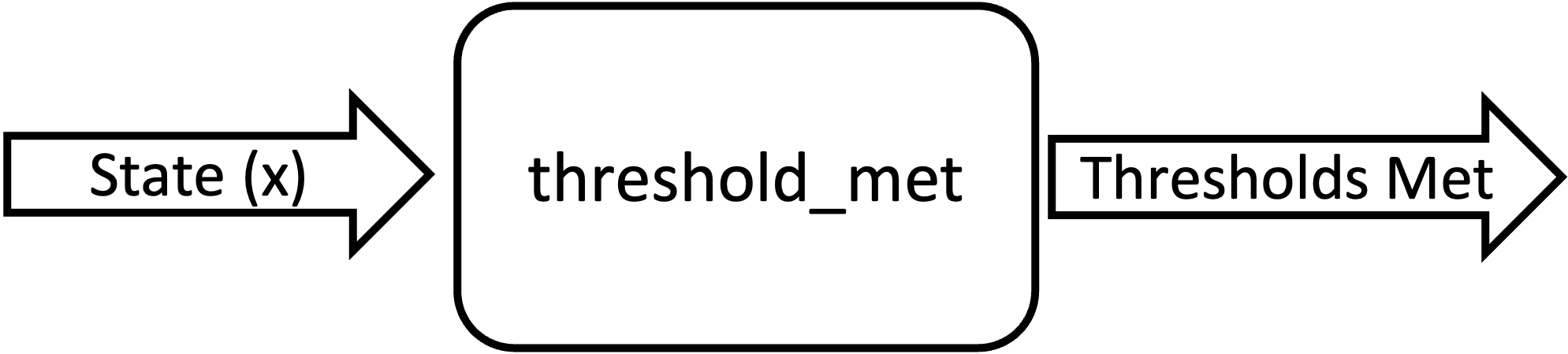
\(tm(t) = f(x(t), \Theta)\)
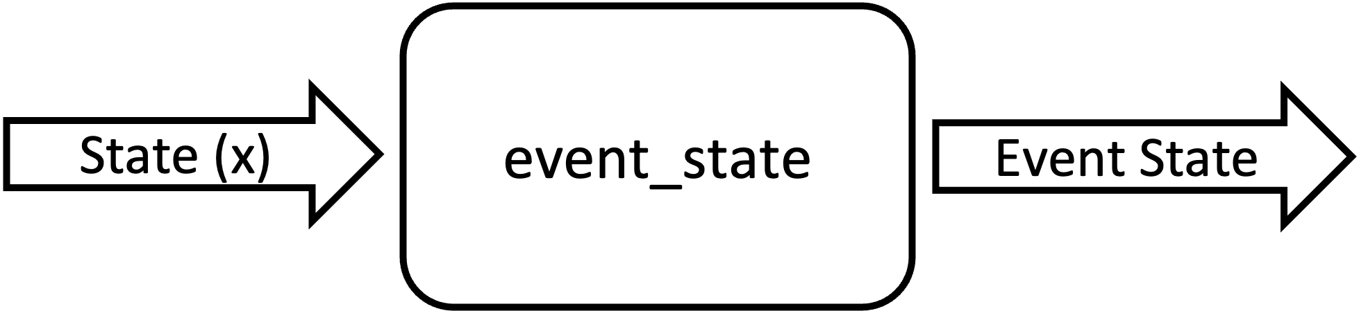
Event states are an estimate of the progress towards a threshold. Where thresholds are boolean, event states are a number between 0 and 1, where 0 means the event has occured, 1 means no progress towards the event. Event states are a generalization of State of Health (SOH) for systems with multiple events and non-failure events. The logic of the event states is defined in progpy.PrognosticsModel.event_state().
\(es(t) = f(x(t), \Theta)\)
If threshold_met is not specified, threshold_met is defined as when event_state is 0. Alternately, if event_state is not defined, it will be 0 when threshold_met is True, otherwise 1. If a model has events, at least one of these methods must be defined
Event Examples
An example of a event_state and threshold_met equations for a thrown object is included below. In this example, a model is created to describe an object thrown directly into the air. It has two states: position (x) and velocity (v). The event_state and threshold_met equations for this example are included below
>>> def event_state(self, x):
>>>     # Falling event_state is 0 when velocity hits 0, 1 at maximum speed
>>>     falling_es = np.maximum(x['v']/self.parameters['throwing_speed'], 0)
>>>
>>>     # Impact event_state is 0 when position hits 0,
>>>     # 1 when at maximum height or when velocity is positive (going up)
>>>     if x['v'] > 0:
>>>         # Event state is 1 until falling starts
>>>         x_max = 1
>>>     else:
>>>         # Use speed and position to estimate maximum height
>>>         x_max = x['x'] + np.square(x['v'])/(-self.parameters['g']*2)
>>>     impact_es = np.maximum(x['x']/x_max,0)
>>>     return {'falling': falling_es, 'impact': impact_es}
>>> def threshold_met(self, x):
>>>     return {
>>>         'falling': x['v'] < 0,
>>>         'impact': x['x'] <= 0
>>>     }
Parameters#
Parameters are used to configure the behavior of a model. For parameterized physics-based models, parameters are used to configure the general system to match the behavior of the specific system. For example, parameters of the general battery model can be used to configure the model to describe the behavior of a specific battery.
Models define a default_parameters property- the default parameters for that model. After construction, the parameters for a specific model can be accessed using the parameters property. For example, for a model m
>>> print(m.parameters)
Parameters can be set in model construction, using the parameters property after construction, or using Parameter Estimation feature (See Parameter Estimation). The first two are illustrated below:
>>> m = SomeModel(some_parameter=10.2, some_other_parameter=2.5)
>>> m.parameters['some_parameter'] = 11.2  # Overriding parameter
The specific parameters are very specific to the system being modeled. For example, a battery might have parameters for the capacity and internal resistance. When using provided models, see the documentation for that model for details on parameters supported.
Derived Parameters
Sometimes users would like to specify parameters as a function of other parameters. This feature is called “derived parameters”. See the derived parameters section in the example below for more details on this feature.
Noise#
In practice, it is impossible to have absolute knowledge of future states due to uncertainties in the system. There is uncertainty in the estimates of the present state, future inputs, models, and prediction methods [Goebel2017]. This model-based prognostic approach incorporates this uncertainty in four forms: initial state uncertainty (\(x_0\)), process noise, measurement noise, and future loading noise.
Process Noise
Process noise is used to represent uncertainty in the state transition process (e.g., uncertainty in the quality of your model or your model configuration parameters).
Process noise is applied in the state transition method (See States).
Measurement Noise
Measurement noise is used to represent uncertainty in your measurements. This can represent such things as uncertainty in the logic of the model’s output method or sensor noise.
Measurement noise is applied in the output method (See Output (Measurements)).
Future Loading Noise
Future loading noise is used to represent uncertainty in knowledge of how the system will be loaded in the future (See Future Loading). Future loading noise is applied by the user in their provided future loading method by adding random noise to the estimated future load.
See the noise section in the example below for details on how to configure proccess and measurement noise in ProgPy.
Future Loading#
Future Loading is an essential part of prediction and simulation. In order to simulate forward in time, you must have an estimate of how the system will be used (i.e., loaded) during the window of time that the system is simulated. Future load is essentially expected Inputs at future times.
Future loading is provided by the user either using the predifined loading classes in progpy.loading, or as a function of time and optional state. For example:
def future_load(t, x=None):
    # Calculate inputs
    return m.InputContainer({'input1': ...})
See the future loading section in the example below for details on how to provide future loading information in ProgPy.
General Notes#
Users of ProgPy will need a model describing the behavior of the system of interest. Users will likely either use one of the models distribued with ProgPy (see Included Models), configuring it to their own system using parameter estimation (see 02 Parameter Estimation), use a data-driven model class to learn system behavior from data, or build their own model (see Building New Models section, below).
Building New Models#
ProgPy provides a framework for building new models. Generally, models can be divided into three basis categories: physics-based models, data-driven models, and hybrid models. Additionally, models can rely on state-transition for prediction, or they can use what is called direct-prediction. These two categories are described below.
State-Transition Models#
New physics-based models are constructed by subclassing progpy.PrognosticsModel as illustrated in the first example. To generate a new model, create a new class for your model that inherits from this class. Alternatively, you can copy the template prog_model_template.ProgModelTemplate, replacing the methods with logic defining your specific model. The analysis and simulation tools defined in progpy.PrognosticsModel will then work with your new model.
For simple linear models, users can choose to subclass the simpler progpy.LinearModel class, as illustrated in the second example. Some methods and algorithms only function on linear models.
New data-driven models, such as those using neural networks, are created by subclassing the progpy.data_models.DataModel class, overriding the from_data method.
The progpy.data_models.DataModel.from_data() and progpy.data_models.DataModel.from_model() methods are used to construct new models from data or an existing model (i.e., surrogate), respectively. The use of these is demonstrated in the following examples.
Note
To use a data-driven model distributed with progpy you need to install the data-driven dependencies.
$ pip install progpy[datadriven]
Advanced features in data models
Direct-Prediction Models#
Direct-prediction models are models that estimate time of event directly from the current state and future load, instead of being predicted through state transition. When models are pure direct-prediction models, future states cannot be predicted. See the direct models section in the example below for more information.
Using Data#
Whether you’re using data-driven, physics-based, expert knowledge, or some hybrid approach, building and validating a model requires data. In the case of data-driven approaches, data is used to train and validate the model. In the case of physics-based, data is used to estimate parameters (see Parameter Estimation) and validate the model.
ProgPy includes some example datasets. See ProgPy Datasets and the example below for details.
Note
To use the dataset feature, you must install the requests package.
Using Provided Models#
ProgPy includes a number of predefined models in the progpy.models module. These models are parameterized, so they can be configured to represent specific systems (see Parameter Estimation).
For details on the included models, see Included Models. The examples below also illustrate the use of some models provided in the progpy.models module.
Simulation#
One of the most basic of functions using a model is simulation. Simulation is the process of predicting the evolution of system state with time, given a specific future load profile. Unlike full prognostics, simulation does not include uncertainty in the state and other product (e.g., output) representation. For a prognostics model, simulation is done using the progpy.PrognosticsModel.simulate_to() and progpy.PrognosticsModel.simulate_to_threshold() methods.
Saving Results
progpy.PrognosticsModel.simulate_to() and progpy.PrognosticsModel.simulate_to_threshold() return the inputs, states, outputs, and event states at various points in the simulation. Returning these values for every timestep would require a lot of memory, and is not necessary for most use cases, so ProgPy provides an ability for users to specify what data to save.
There are two formats to specify what data to save: the save_freq and save_pts arguments, described below
Argument |
Description |
Example |
|---|---|---|
|
The frequency at which data is saved |
|
|
Specific times at which data is saved |
|
Note
Data will always be saved at the next time after the save_pt or save_freq. As a result, the data may not correspond to the exact time specified. Use automatic step sizes to save at the exact time.
Step Size
Step size is the size of the step taken in integration. It is specified by the dt argument. It is an important consideration when simulating. Too large of a step size could result in wildly incorrect results, and two small of a step size can be computationally expensive. Step size can be provided in a few different ways, described below:
Static Step Size: Provide a single number. Simulation will move forward at this rate. Example,
m.simulate_to_threshold(..., dt=0.1)Automatic Dynamic Step Size: Step size is adjusted automatically to hit each save_pt and save_freq exactly. Example,
m.simulate_to_threshold(..., dt='auto')Bounded Automatic Dynamic Step Size: Step size is adjusted automatically to hit each save_pt and save_freq exactly, with a maximum step size. Example,
m.simulate_to_threshold(..., dt=('auto', 0.5))Functional Dynamic Step Size: Step size is provided as a function of time and state. This is the most flexible approach. Example,
m.simulate_to_threshold(..., dt= lambda t, x : max(0.75 - t*0.01, 0.25))
For more details on dynamic step sizes, see the following example:
Integration Methods
Simulation is essentially the process of integrating the model forward with time. By default, simple euler integration is used to propogate the model forward. Advanced users can change the numerical integration method to affect the simulation quality and runtime. This is done using the integration_method argument in progpy.PrognosticsModel.simulate_to_threshold() and progpy.PrognosticsModel.simulate_to().
For example, users can use the commonly-used Runge Kutta 4 numerical integration method using the following method call for model m:
>>> m.simulate_to_threshold(future_loading, integration_method = 'rk4')
Eval Points
Sometimes users would like to ensure that simulation hits a specific point exactly, regardless of the step size (dt). This can be done using the eval_pts argument in progpy.PrognosticsModel.simulate_to_threshold() and progpy.PrognosticsModel.simulate_to(). This argument takes a list of times at which simulation should include. For example, for simulation to evaluate at 10 and 20 seconds, use the following method call for model m:
>>> m.simulate_to_threshold(future_loading, eval_pts = [10, 20])
This feature is especially important for use cases where loading changes dramatically at a specific time. For example, if loading is 10 for the first 5 seconds and 20 afterwards, and you have a dt of 4 seconds, here’s loading simulation would see:
0-4 seconds: 10
4-8 seconds: 10
8-12 seconds: 20
That means the load of 10 was applied 3 seconds longer than it was supposed to. Adding a eval point of 5 would apply this load:
0-4 seconds: 10
4-5 seconds: 10
5-9 seconds: 20
Now loading is applied correctly.
For simulation examples, see the following notebook for details.
Parameter Estimation#
Parameter estimation is an important step in prognostics. Parameter estimation is used to tune a general model to match the behavior of a specific system. For example, parameters of the general battery model can be used to configure the model to describe the behavior of a specific battery.
Sometimes model parameters are directly measurable (e.g., dimensions of blades on rotor). For these parameters, estimating them is a simple act of direct measurement. For parameters that cannot be directly measured, they’re typically estimated using observed data.
Generally, parameter estimation is done by tuning the parameters of the model so that simulation best matches the behavior observed in some available data. In ProgPy, this is done using the progpy.PrognosticsModel.estimate_params() method. This method takes input and output data from one or more runs, and uses scipy.optimize.minimize function to estimate the parameters of the model.
>>> params_to_estimate = ['param1', 'param2']
>>> m.estimate_params([run1_data, run2_data], params_to_estimate, dt=0.01)
See the example below for more details.
Note
Parameters are changes in-place, so the model on which estimate_params is called, is now tuned to match the data.
Visualizing Results#
Results of a simulation can be visualized using the plot method. For example:
>>> results = m.simulate_to_threshold(...)
>>> results.outputs.plot()
>>> results.states.plot()
See progpy.sim_result.SimResult.plot() for more details on plotting capabilities
Combination Models#
There are two methods in progpy through which multiple models can be combined and used together: composite models and ensemble models, described below. For more details, see the example below.
Composite models are used to represent the behavior of a system of interconnected systems. Each system is represented by its own model. These models are combined into a single composite model which behaves as a single model. When definiting the composite model the user provides a discription of any connections between the state or output of one model and the input of another. For example,
>>> m = CompositeModel(
>>>     models = [model1, model2],
>>>     connections = [
>>>         ('model1.state1', 'model2.input1'),
>>>         ('model2.state2', 'model1.input2')
>>>     ]
>>> )
Unlike composite models which model a system of systems, ensemble models are used when to combine the logic of multiple models which describe the same system. This is used when there are multiple models representing different system behaviors or conditions. The results of each model are aggregated in a way that can be defined by the user. For example,
>>> m = EnsembleModel(
>>>     models = [model1, model2],
>>>     aggregator = np.mean
>>> )
Mixture of Experts (MoE) models combine multiple models of the same system, similar to Ensemble models. Unlike Ensemble Models, the aggregation is done by selecting the “best” model. That is the model that has performed the best over the past. Each model will have a ‘score’ that is tracked in the state, and this determines which model is best.
>> m = MixtureOfExpertsModel([model1, model2])
Other Examples#
Tips & Best Practices#
If you’re only doing diagnostics without prognostics- just define a next_state equation with no change of state and don’t perform prediction. The state estimator can still be used to estimate if any of the events have occured.
Sudden events use a binary event state (1=healthy, 0=failed).
You can predict as many events as you would like, sometimes one event must happen before another, in this case the event occurance for event 1 can be a part of the equation for event 2 (‘event 2’: event_1 and [OTHER LOGIC]).
Minimize the number of state variables whenever possible
Whenever possible, if calculations dont include state or inputs, include values as parameters or derived parameters instead of calculating within state transition
Use constant units throughout the model
Document all assumptions and limitations
References#
- Goebel2017
Kai Goebel, Matthew John Daigle, Abhinav Saxena, Indranil Roychoudhury, Shankar Sankararaman, and José R Celaya. Prognostics: The science of making predictions. 2017
- Celaya2012
J Celaya, A Saxena, and K Goebel. Uncertainty representation and interpretation in model-based prognostics algorithms based on Kalman filter estimation. Annual Conference of the Prognostics and Health Management Society, 2012.
- Sankararaman2011
S Sankararaman, Y Ling, C Shantz, and S Mahadevan. Uncertainty quantification in fatigue crack growth prognosis. International Journal of Prognostics and Health Management, vol. 2, no. 1, 2011.