6.1.2. OVERFLOW Powered Nacelle Example
This pyOver example shows how to use pyover to run one of the simple test
cases that come with the OVERFLOW source code. This example starts with the
grids and inputs files that are created within the OVERFLOW examples, and
documents how to create the pyOver setup, run matrix, how to run several
OVERFLOW cases, covers some post-processing. This example is located in a
git repo. After cloning this repo, enter the resulting folder
$ git clone https://github.com/nasa-ddalle/pyover02-powered_nacelle.git
$ cd pyover02-powered_nacelle
the folder has the required input files, but it’s recommended to copy them to a working folder so that it’s easy to reset. Just run the following command:
$ ./copy_files.py
$ cd work/
This example shows how to use pyOver for a test case with two related configurations, a flow-through axisymmetric nacelle, and a powered axisymmetric nacelle. The example comes with the grids and input files ready to run OVERFLOW.
6.1.2.1. Flow-Through Nacelle Case
Given the grid and input files created by the OVERFLOW scripts, the only two
files that are required to run the flow-through example using pyOver are
flowthrough.json and inputs/matrix/flowthrough.csv.
To execute and duplicate the OVERFLOW Mach 0.8 flow-through example, simply run
the command pyover -f flowthrough.json -I 1. This simple problem
will run in a matter of seconds:
pyover -f flowthrough.json -I 1
Case Config/Run Directory  Status  Iterations  Que CPU Time
---- --------------------- ------- ----------- --- --------
1    flowthrough/m0.8      ---     /           .
  Case name: 'flowthrough/m0.8' (index 1)
     Starting case 'flowthrough/m0.8'
 > overrunmpi -np 8 run 01
     (PWD = 'flowthrough/m0.8')
     (STDOUT = 'overrun.out')
   Wall time used: 0.00 hrs (phase 0)
   Wall time used: 0.00 hrs
   Previous phase: 0.00 hrs
 > overrunmpi -np 8 run 02
     (PWD = 'flowthrough/m0.8')
     (STDOUT = 'overrun.out')
   Wall time used: 0.00 hrs (phase 1)

Submitted or ran 1 job(s).

---=1,
This ran the MPI version of OVERFLOW locally, (without submitting a PBS job or similar) using 8 processors (cores). The actions that pyOver takes are summarized here:
Create the directory
flowthrough/m0.8/Create symbolic links pointing to some files in
common_flowthroughCreate two OVERFLOW inputs files
run.01.inpandrun.02.inpExecute
overrunmpi -np 8 run 01Execute
overrunmpi -np 8 run 02
The sections in flowthrough.json that control the execution of
OVERFLOW are shown here:
// Namelist template
"OverNamelist": "common_flowthrough/overflow.inp",
// Options for overall run control and command-line inputs
"RunControl": {
    // Run sequence
    "PhaseSequence": [0,   1],
    "PhaseIters":    [600, 1400],
    // Operation modes
    "Prefix": "run",
    "MPI": true,
    "qsub": false,
    "Resubmit": [false, true],
    "Continue": true,
    "mpicmd": null,
    "nProc": 8,
    // Dictionary of environment variables
    "Environ": {
        "F_UFMTENDIAN": "little"
    },

    // OVERFLOW command-line interface
    "overrun": {
        "cmd": "overrunmpi",
        "aux": null
    }
},
The PhaseSequence and PhaseIters specify how many times and how long the
code is run. The first specifies that OVERFLOW will run for phase 0 and
phase 1, (which are labeled as 01 and 02 for overrunmpi
execution). These phases run until there are 600 and 1400 total global steps
in OVERFLOW. For these and other inputs in the .json file, the sequential
list of arguments are applied to sequentially to each phase. Note that
if only one value is given, that value is applied for all phases. Also note
that if the number of phases are greater than the number of inputs in a
sequential list, the latter phases will use the last value given in the list.
Setting MPI to true instructs pyOver to use the MPI version
of OVERFLOW, but setting mpicmd to null is required because we want
pyOver to use the overrunmpi script, as specified by the cmd value in
the overrun section.
Note that the actual number of iterations in one run of each phase is not set
in the RunControl section above. These are controlled by the OVERFLOW input
variable NSTEPS in the GLOBAL namelist. In the first phase we are also
running full-multi-grid (FMG) iterations with FMGCYC = [[300, 300]] and
NSTEPS[0] = 0, thus 600 total iterations in the first phase.
Here are the sections in flowthrough.json that control the GLOBAL
and OMIGLB namelists:
// Namelist inputs
"Overflow": {
    "GLOBAL": {
        "NQT": 102,
        "NSTEPS": [0,   800],
        "NSAVE":  [0,  2000],
        "FMG": [true, false],
        "FMGCYC": [[300,300]],
        "NGLVL": 3,
        "ISTART_QAVG": 15000,
        "WALLDIST": [2],
        "DTPHYS": [0.0, 0.0, 0.0, 0.0, 1.0],
        "NITNWT": [0,   0,   0,     0,   5]
    },
    "OMIGLB": {
        "IRUN": 0
    }
},
Here are the sections in flowthrough.json that control the namelists
for each individual mesh. The “ALL”: section is applied to all grids.
If one wants to specify different input values for a single grid, duplicate
this section and replace “ALL” with the name of that grid in double quotes.
// Namelist parameters for each grid
"Grids": {
    // Settings applied to all grids
    "ALL": {
        // Solver parameters
        "METPRM": {
            "IRHS": 0,
            "ILHS": 2
        },
        "TIMACU": {
            "ITIME": 1,
            "DT": 0.10,
            "CFLMIN": 5.0,
            "CFLMAX": 0.0
        },
        "SMOACU": {
            "DIS2": 2.0,
            "DIS4": 0.04,
            "DELTA": 1.0
        }
    }
},
Here is the MESH section, which tells pyOver which files to copy and which files to create symbolic links for.
// Mesh
"Mesh": {
    // Folder containing definition files
    "ConfigDir": "common_flowthrough",
    // Grid type, dcf or peg5
    "Type": "dcf",
    // List or dictionary of files to link
    "LinkFiles": [
        "grid.in",
        "xrays.in",
        "fomo/grid.ib",
        "fomo/grid.ibi",
        "fomo/grid.nsf",
        "fomo/grid.map"
    ],
    // List of files to copy instead of linking
    "CopyFiles": [
        "Config.xml",
        "fomo/mixsur.fmp"
    ]
},
One very important section of flowthrough.json is the RunMatrix
section, shown here:
// RunMatrix description
"RunMatrix": {
    // If a file is specified, and it exists, trajectory values will be
    // read from it.  RunMatrix values can also be specified locally.
    "File": "inputs/matrix/flowthrough.csv",
    "Keys": ["mach"],
    // Copy the mesh
    "GroupMesh": true,
    // Configuration name [default]
    "GroupPrefix": "flowthrough"
}
This describes an extremely simple run matrix file, whose only primary input variable (listed in the Keys input) is mach. Because the flow-through nacelle is an axisymmetric flow problem, one cannot run different angles of incidence, therefore alpha and beta are not listed as input variables.
6.1.2.2. Run Mach Sweep
Having defined the RunMatrix section in the json file, we can see that the
run matrix given in the inputs/matrix/flowthrough.csv file looks
like this:
# mach, config, Label
  0.75, flowthrough,
  0.80, flowthrough,
  0.85, flowthrough,
  0.90, flowthrough,
The run matrix consists of four cases with different Mach numbers. These cases
can all be run using just the command pyover. Doing this will execute the
three remaining cases (since we ran case 1 in the beginning). Afterwards,
check the status of the cases using pyover -c, which should produce a list
showing all the cases with a status of DONE:
Case Config/Run Directory  Status  Iterations  Que CPU Time
---- --------------------- ------- ----------- --- --------
0    flowthrough/m0.75     DONE    1400/1400   .        0.0
1    flowthrough/m0.8      DONE    1400/1400   .        0.0
2    flowthrough/m0.85     DONE    1400/1400   .        0.0
3    flowthrough/m0.9      DONE    1400/1400   .        0.0

DONE=4,
6.1.2.3. Report Generation
After running all four cases in the run matrix, the next thing to do is examine the convergence and view the flow. This can be accomplished for our case using the command:
pyover --report -I 0:4
This will create the report in the file report/report-flowthrough.pdf.
There should be two pages for each case, one page with a table of aerodynamic
data and several convergence plots, and one page with two flow-visualization
figures.
6.1.2.3.1. Convergence Plots
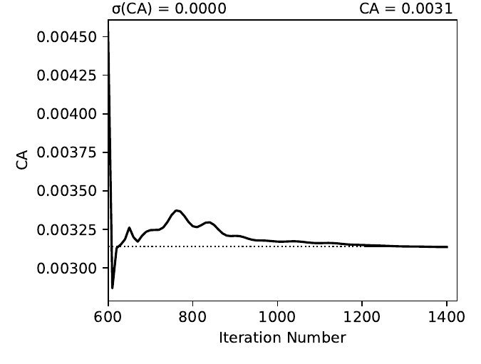
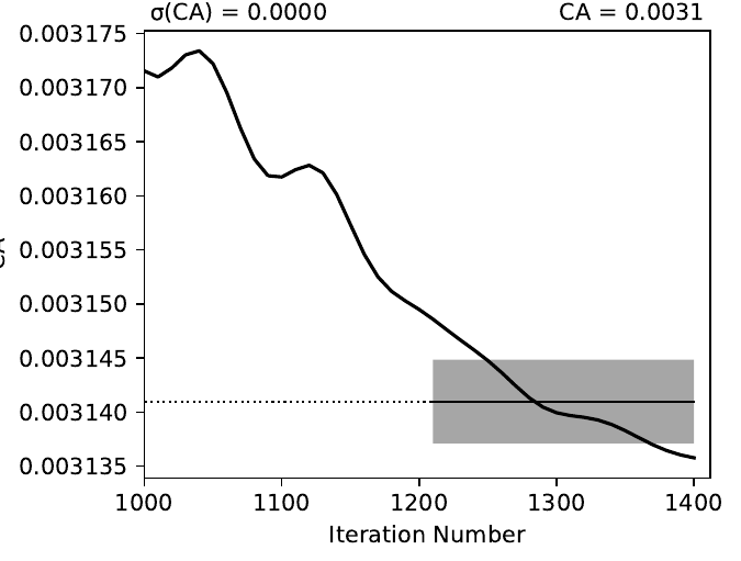
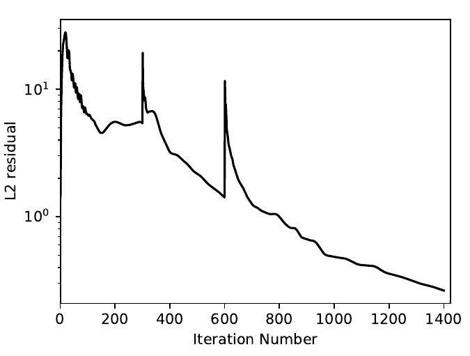
Nine different convergence plots are shown on the first page of the report for
each case. In addition to plotting the history of the three force coefficients
and the three moment coefficients, the plot of the residual history, two
different views are added zooming into the tail end of the axial force
coefficient convergence. The force_CAzoom1 and force_CAzoom2 subfigures
show the last 800 and last 400 iterations of the convergence history.
The definition of the subfigures used to view the convergence is relatively
straightforward. The following shows the these subfigure definitions in
flowthrough.json:
// Definitions for subfigures
"Subfigures": {
    ...
    ...
    // Iterative history
    "force": {
        "Type": "PlotCoeff",
        "Component": "TOTAL FORCE",
        "nPlotFirst": 0,
        "FigWidth": 4.5,
        "FigHeight": 3.4,
        "Width": 0.33,
        "StandardDeviation": 1.0
    },
    "force_CA": {"Type": "force", "Coefficient": "CA"},
    "force_CY": {"Type": "force", "Coefficient": "CY"},
    "force_CN": {"Type": "force", "Coefficient": "CN"},
    "force_CLL": {"Type": "force", "Coefficient": "CLL"},
    "force_CLM": {"Type": "force", "Coefficient": "CLM"},
    "force_CLN": {"Type": "force", "Coefficient": "CLN"},
    "force_CAzoom1": {
        "Type": "force",
        "Coefficient": "CA",
        "nPlotFirst": -800
    },
    "force_CAzoom2": {
        "Type": "force",
        "Coefficient": "CA",
        "nPlotFirst": -400
    },
    // Residual history
    "L2": {
        "Type": "PlotL2",
        "FigWidth": 5.5,
        "FigHeight": 6,
        "Width": 0.33,
        "nPlotFirst": 1,
        "Caption": "$L_2$ Density Residual"
    }
}
When viewing the convergence and showing the entire history it can appear that the forces are very tightly converged. But when viewing the tail end, one can see that the axial force is still dropping slightly. The following figures show four of the convergence plots illustrating the three views of CA as well as the history of the L2 norm of the residual of the mean-flow quantities.
Table 6.3 Convergence plots for the m0.75 case¶ 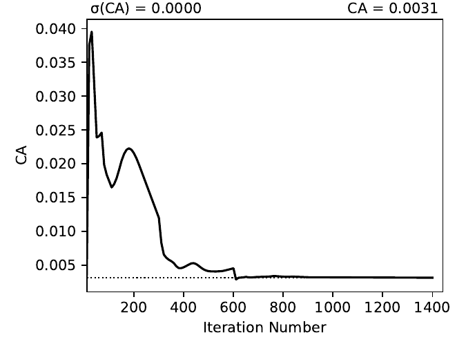
TOTAL FORCE/CA
TOTAL FORCE/CA
TOTAL FORCE/CA
L2 Residual
6.1.2.3.2. Flow Visualization
In the Report section of flowthrough.json, the subfigures for the
flow visualization use Tecplot® subfigures. Here we re-use the contour and
color map settings from the 01-bullet pyover example. The MachSlice
subfigure uses tecplot and the supplied layout file in
inputs/flowthrough-mach.lay to create Mach contours in the Y=0 plane
of the nacelle. Note that the MaxLevel for the contours is dependant
upon the freestream Mach number. The color map break points are also a function
of the freestream Mach.
At the end of this section, the MachSlice-mesh subfigure is defined. This subfigure inherits all of the settings from the MachSlice subfigure, but uses a different layout file. The only difference between the two layout files is that the addition of the mesh overlay on the Mach contours.
// Definitions for subfigures
"Subfigures": {
    // Tecplot figures
    "MachSlice": {
        "Type": "Tecplot",
        "Layout": "inputs/flowthrough-mach.lay",
        "FigWidth": 1024,
        "Width": 0.65,
        "Caption": "Mach slice $y=0$",
        "ContourLevels": [
            {
                "NContour": 1,
                "MinLevel": 0,
                "MaxLevel": "max(1.4, 1.4*$mach)",
                "Delta": 0.05
            }
        ],
        "ColorMaps": [
            {
                "Name": "Diverging - Purple/Green modified",
                "NContour": 2,
                "ColorMap": {
                    "0.0": "purple",
                    "$mach": "white",
                    "1.0": ["green", "orange"],
                    "max(1.4,1.4*$mach)": "red"
                }
            }
        ],
        "Keys": {
            "GLOBALCONTOUR": {
                "LABELS": {
                    "Value": {
                        "AUTOLEVELSKIP": 2,
                        "NUMFORMAT": {
                            "FORMATTING": "'FIXEDFLOAT'",
                            "PRECISION": 1,
                            "TIMEDATEFORMAT": "''"
                        }
                    },
                    "Parameter": 1
                }
            }
        }
    },
    "MachSlice-mesh": {
        "Type": "MachSlice",
        "Layout": "inputs/flowthrough-mach-mesh.lay"
    },
  ...
  ...
}
The resulting MachSlice subfigures for each of the four cases are shown here:
Table 6.4 Tecplot® Mach contour plots for each case¶ 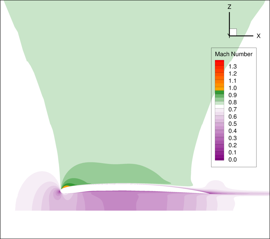
Mach slice m0.75
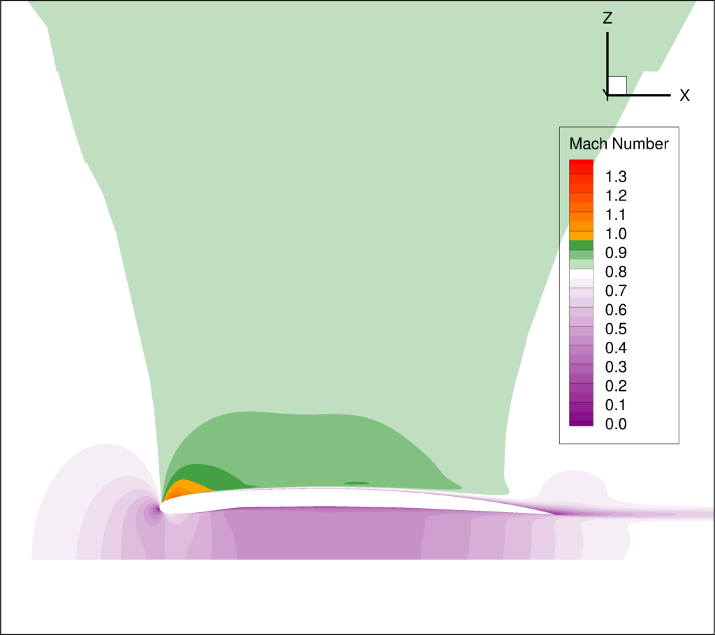
Mach slice m0.80

Mach slice m0.80
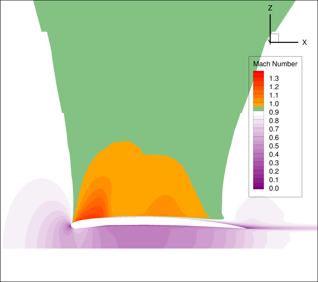
Mach slice m0.90
6.1.2.4. Powered Nacelle Cases
The powered nacelle test cases that come with Overflow also include three cases simulating the effect of an engine inside of the nacelle. This adds two boundaries inside of the nacelle. The first simulates the effect of the forward fan face in the inlet side of the nacelle. At this boundary the air is flowing out of the CFD domain. The second boundary simulates the flow exiting the engine. At this boundary the air is flowing into the CFD domain.
6.1.2.4.1. pyover Setup
To create this test case in pyover, we have created these new files:
powered.json
inputs/matrix/powered.csv
inputs/powered-mach.lay
inputs/powered-mach-mesh.lay
These were created by merely copying the flowthrough versions of the files and making slight modifications. You can compare the powered with the flowthrough versions of each file to see the modifications that were made. However, there is one more step, and it requires something new.
Note that three different overflow input files are provided in the OVERFLOW source code for this case. These three input files have been installed in the pyover example as:
common_powered/overflow_test01.inp
common_powered/overflow_test02.inp
common_powered/overflow_test03.inp
The basic pyover setup only allows one to specify one OVERFLOW input file for
the template input file, but we have three different input files that we want
to use. This example will show how to incorporate a python module that will
customize the behavior of pyover in order to specify different OVERFLOW input
files. To enable this we will make use of the Label column in the input
run matrix file. The Label values will be used in the naming of the
run directories. Here are the first four lines in the input file:
inputs/matrix/powered.csv.
# mach, config,  Label
  0.80, powered, test01
  0.80, powered, test02
  0.80, powered, test03
Here is the corresponding RunMatrix entry in the powered.json file:
// RunMatrix description
"RunMatrix": {
    // If a file is specified, and it exists, trajectory values will be
    // read from it.  RunMatrix values can also be specified locally.
    "File": "inputs/matrix/powered.csv",
    "Keys": ["mach", "config", "Label"],
    // Copy the mesh
    "GroupMesh": true,
    // Configuration name [default]
    "GroupPrefix": "powered"
}
In order to customize the pyover behavior, we have added some python code
in a file called tools/nacelle.py, and have added these lines to the
powered.json file:
// Module settings
"PythonPath": ["tools"],
"Modules": ["nacelle"],
"InitFunction": ["nacelle.InitNAC1"],
"CaseFunction": ["nacelle.ApplyLabel"],
This notifies pyover to look in the tools directory for a python module
called nacelle.py. It also identifies two functions in the nacelle.py
module that will be executed by pyover. The first function InitNac1() will
be called when pyover first starts running. The second function ApplyLabel
will be called during the process of creating each of the runs. These two
functions have been written in the tools/nacelle.py file. The
InitNac1() does not actually do anything in this example, but this function
can be used customize certain behaviors at the beginning of a pyover run. The
ApplyLabel() function is shown here:
# Apply options based on the *Label* RunMatrix key
def ApplyLabel(cntl, i):
    """Modify settings for each case using value of *Label*

    This method is programmed to specify a different OVERFLOW input
    file based on the value of *Label* for a given case. This is used
    to run each of the three input files that come with the
    powered_nacelle test problem that comes with the OVERFLOW source
    code.

    :Call:
        >>> ApplyLabel(cntl, i)
    :Inputs:
        *cntl*: :class:`pyOver.overflow.Overflow`
            OVERFLOW settings interface
        *i*: :class:`int`
            Case number
    :Versions:
        * 2020-01-28 ``@serogers``: First version
    """

    # Get the specified label
    lbl = cntl.x['Label'][i]
    # Set the overflow input file as a function of the Label
    if 'test01' in lbl:
        cntl.opts['OverNamelist'] = 'common_powered/overflow_test01.inp'
    elif 'test02' in lbl:
        cntl.opts['OverNamelist'] = 'common_powered/overflow_test02.inp'
    elif 'test03' in lbl:
        cntl.opts['OverNamelist'] = 'common_powered/overflow_test03.inp'
6.1.2.4.2. Executing pyover
This completes the setup, the next step is to run pyover and run all three test cases:
> pyover -f powered.json
Importing module 'nacelle'
  InitFunction: nacelle.InitNAC1()
Case Config/Run Directory  Status  Iterations  Que CPU Time
---- --------------------- ------- ----------- --- --------
0    powered/m0.8_test01   ---     /           .
  Case Function: cntl.nacelle.ApplyLabel(0)
  Case name: 'powered/m0.8_test01' (index 0)
     Starting case 'powered/m0.8_test01'
 > overrunmpi -np 8 run 01
     (PWD = '/u/wk/serogers/usr/cape/examples/pyover/02_powered_nacelle/powered/m0.8_test01')
     (STDOUT = 'overrun.out')
   Wall time used: 0.00 hrs (phase 0)
   Wall time used: 0.00 hrs
   Previous phase: 0.00 hrs
 > overrunmpi -np 8 run 02
     (PWD = '/u/wk/serogers/usr/cape/examples/pyover/02_powered_nacelle/powered/m0.8_test01')
     (STDOUT = 'overrun.out')
   Wall time used: 0.00 hrs (phase 1)
1    powered/m0.8_test02   ---     /           .
  Case Function: cntl.nacelle.ApplyLabel(1)
  Case name: 'powered/m0.8_test02' (index 1)
     Starting case 'powered/m0.8_test02'
 > overrunmpi -np 8 run 01
     (PWD = '/u/wk/serogers/usr/cape/examples/pyover/02_powered_nacelle/powered/m0.8_test02')
     (STDOUT = 'overrun.out')
   Wall time used: 0.00 hrs (phase 0)
   Wall time used: 0.00 hrs
   Previous phase: 0.00 hrs
 > overrunmpi -np 8 run 02
     (PWD = '/u/wk/serogers/usr/cape/examples/pyover/02_powered_nacelle/powered/m0.8_test02')
     (STDOUT = 'overrun.out')
   Wall time used: 0.00 hrs (phase 1)
2    powered/m0.8_test03   ---     /           .
  Case Function: cntl.nacelle.ApplyLabel(2)
  Case name: 'powered/m0.8_test03' (index 2)
     Starting case 'powered/m0.8_test03'
 > overrunmpi -np 8 run 01
     (PWD = '/u/wk/serogers/usr/cape/examples/pyover/02_powered_nacelle/powered/m0.8_test03')
     (STDOUT = 'overrun.out')
   Wall time used: 0.00 hrs (phase 0)
   Wall time used: 0.01 hrs
   Previous phase: 0.00 hrs
 > overrunmpi -np 8 run 02
     (PWD = '/u/wk/serogers/usr/cape/examples/pyover/02_powered_nacelle/powered/m0.8_test03')
     (STDOUT = 'overrun.out')
   Wall time used: 0.00 hrs (phase 1)

Submitted or ran 3 job(s).

---=3,
Note that the output informs you that it is excuting the Case Function
cntl.nacelle.ApplyLabel() before each case is run, passing the case number
as the argument.
6.1.2.4.3. Report Generation
Generate the report for these three cases using pyover -f powered.json
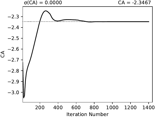
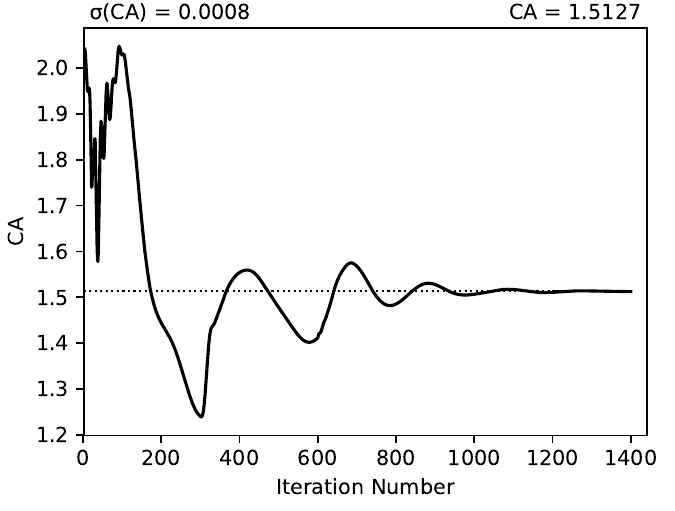
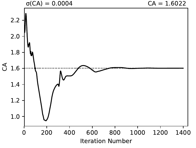
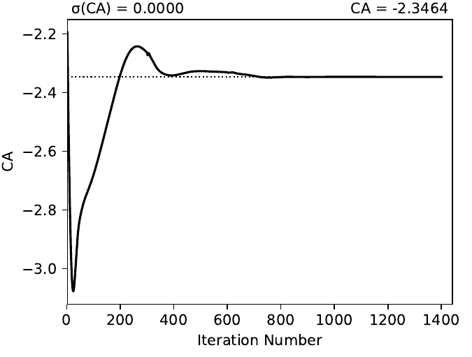
--report. The powered runs plot different convergence history plots than the
flowthrough example. The plots now include the axial force coefficient for
both the INLET and the EXIT components. At this time, pyover does not have
the capability to plot convergence history for the mass-flow rate.
Convergence plots for the INLET and EXIT axial force coefficients for each of the three case are shown here.
Table 6.5 Convergence plots for INLET and EXIT axial force¶ 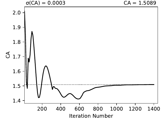
INLET/CA test01
EXIT/CA test01
INLET/CA test02

EXIT/CA test02
INLET/CA test03
EXIT/CA test03
The report also includes MachSlice subfigures. Each case shows the Mach contours with and without the grid included. All three test cases show very similar Mach contours, the subfigures for test01 are shown here:
Table 6.6 Tecplot® Mach contour plots for test01¶ 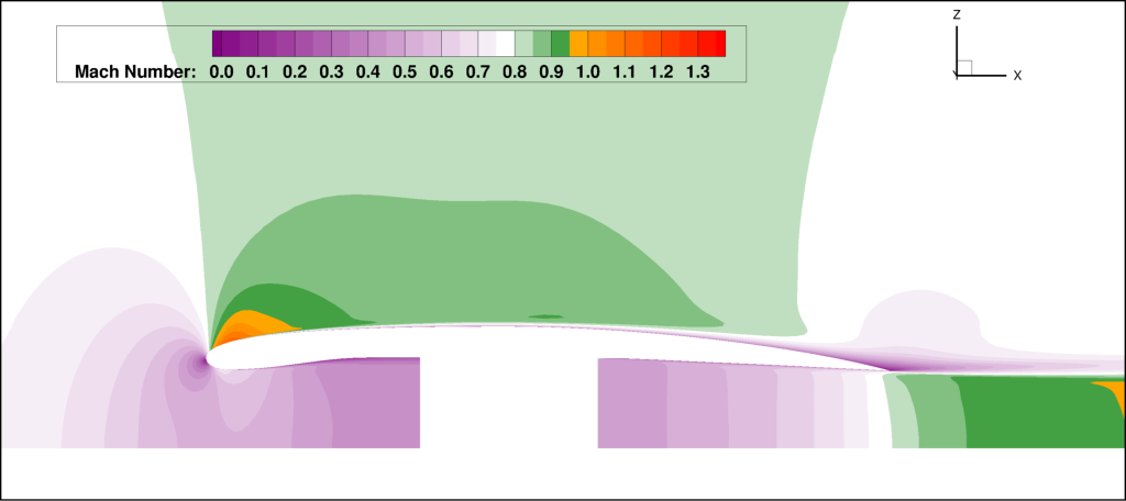
Mach slice test01
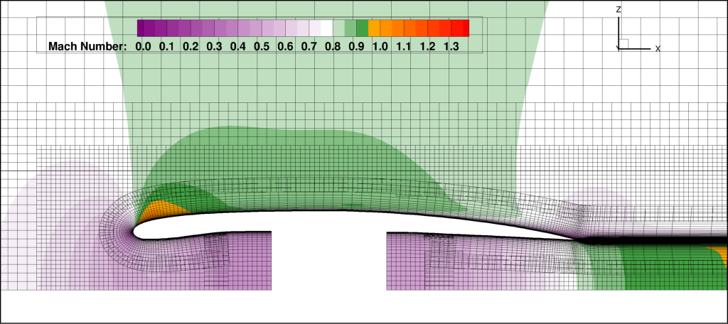
Mach slice with grid
6.1.2.5. Powered Boundary Conditions
This example comes with one more configuration using the powered-nacelle setup that comes with OVERFLOW. This configuration illustrates the ability to manipulate the nacelle boundary conditions in the run matrix file. This can be very useful for developing simulations where the thrust or engine conditions are changed as part of the run matrix. This configuration setup uses the following files:
inputs/matrix/bcpower.json
bcpower.json
tools/bcpower.py
The inputs/matrix/bcpower.json file contains the new run matrix. This file
contains the following:
# mach, InletBC, ExitBC, config,   Label
  0.80, 1.258,    1.200,  bcpower, test01
  0.80, 1.358,    2.000,  bcpower, test01
  0.80, 1.458,    4.000,  bcpower, test01
This has added two new columns called InletBC and ExitBC. These are defined
in the RunMatrix section in the bcpower.json file:
// RunMatrix description
"RunMatrix": {
    "File": "inputs/matrix/bcpower.csv",
    "Keys": ["mach", "InletBC", "ExitBC", "config", "Label"],
    // Copy the mesh
    "GroupMesh": true,
    // Configuration name [default]
    "GroupPrefix": "powered",
    "Definitions": {
        // InletBC
        "InletBC": {
            "Type": "CaseFunction",
            "Function": "self.bcnacelle.ApplyInletBC",
            "Value": "float",
            "Label": true,
            "Format": "%05.3f_",
            "Abbreviation": "I",
            "Grids": "Inlet"
        },
        // ExitBC
        "ExitBC": {
            "Type": "CaseFunction",
            "Function": "self.bcnacelle.ApplyExitBC",
            "Value": "float",
            "Label": true,
            "Format": "%05.3f",
            "Abbreviation": "E",
            "Grids": "Exit"
        }
    }
}
The new columns are assigned the with "Type": "CaseFunction", and has
an attribute assigned for "Function". This will cause
pyover to execute that function when it is time to build the OVERFLOW
input file for each case. It will pass the value from the column in the
RunMatrix to that function for each individual case. Thus when it starts the
first case, it will pass a value of 1.258 to the bcnacelle.ApplyInletBC
function. This is a user-defined function that is located in the
tools/bcnacelle.py python module. Let us examine the contents of this
function:
def ApplyInletBC(cntl, v, i):
    """Modify BCINP for nacelle inlet face

    This method is modifies the BCINP namelist in the OVERFLOW input file
    for the boundary conditions on the Inlet grid

    The IBTYP=33 boundary condition applies a contant pressure outflow
    at the engine inlet face. This uses the value of BCPAR1 to set the
    ratio of the boundary static pressure to freestream pressure.

    The IBTYP=34 boundary condition applies a constant mass-flow rate
    at the engine inlet face. This uses the value of BCPAR1 to set the
    target mass-flow rate.  BCPAR2 sets the update rate and relaxation factor.
    BCFILE is used to supply the FOMOCO component and Aref.

    :Call:
        >>> ApplyInletBC(cntl, v, i)
    :Inputs:
        *cntl*: :class:`pyOver.overflow.Overflow`
            OVERFLOW settings interface
        *v*: :class:`float`
            Run-matrix value in the InletBC column for case i
        *i*: :class:`int`
            Case number
    :Versions:
        * 2020-01-30 ``@serogers``: First version
    """

    ## Inlet grid: set boundary conditions
    grid = 'Inlet'
    bci = 3
    print("\n\nIn function ApplyInletBC, v = ", v)
    # Extract the BCINP from the template for this grid
    IBTYP = cntl.Namelist.GetKeyFromGrid(grid, 'BCINP', 'IBTYP')

    #################################################
    # Process the pressure BC
    if IBTYP.count(33) > 0:
        # Get the column for ibtyp=33
        bci = IBTYP.index(33)
        # Change bci to 1-based index
        bci += 1
        # Set the BCPAR1 value for this case
        cntl.Namelist.SetKeyForGrid(grid, 'BCINP', 'BCPAR1', v, i=bci)
        BCPAR1 = cntl.Namelist.GetKeyFromGrid(grid, 'BCINP', 'BCPAR1', i=bci)
This function is programmed to change the value of BCPAR1 associated with the boundary condition entry that uses IBTYP=33 for the grid named Inlet in the OVERFLOW input file. For IBTYP=33, the BCPAR1 value is used to set the static pressure ratio at an outflow boundary. In other words, it sets the static pressure at the boundary of the engine fan face in our nacelle example. The run matrix is set up to run three different values of static-pressure ratio for the three different cases.
Note that the ApplyInletBC function only changes the boundary condition
if it finds an entry with IBTYP=33 in the OVERFLOW template input file.
It is left as an exercise to the reader to add python code that will change
the boundary condition if IBTYP=34, which controls the mass-flow rate instead
of the pressure.
Similarly, the run-matrix column for ExitBC is tied to a function called
ApplyExitBC, contained in the tools/bcnacelle.py file. This function
sets the value of BCPAR1 for the IBTYP=141 boundary condition. This sets
the total pressure value used at the boundary condition for the nacelle
exit. By varying the values in the ExitBC column of the run matrix, this
changes the total pressure in the flow coming out of the engine, changing
the resulting engine thrust.
The commands to run the three cases and generating the report for this configuration are:
pyover -f bcpower.json -I 0,1,2
pyover -f bcpower.json --report
The report is setup to create the same force and moment convergence plots as
the powered.json configuration. The flow-field contour plots include the
same Mach contour figures, and additionally a figure of pressure coefficient
(Cp) contours. The effect of the changes of the Inlet and Exit boundary conditions
are illustrated in these contour plots. The following table combines the
Cp and Mach contour images for the three cases for each comparison.
The change to flow into the inlet is seen for the InletBC values of 1.258, 1.358, and 1.458. The increasing static pressure on the boundary can be seen in the Cp contours, and its effect of reducing the Mach number of the flow into the inlet boundary.
The total pressure values of 1.2, 2.0, and 4.0 prescribed in the run matrix in the ExitBC column are also evident. The increasing total pressure creates higher exit pressures and higher Mach numbers as the flow exits the nacelle.
Table 6.7 Tecplot® Cp and Mach contour plots for each case¶ 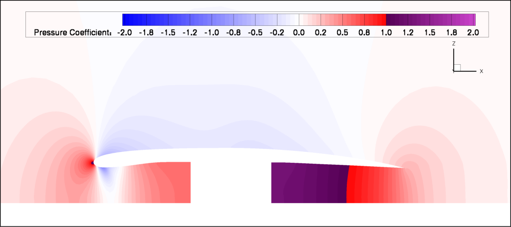
Cp slice bc_power_1.258_E1.200
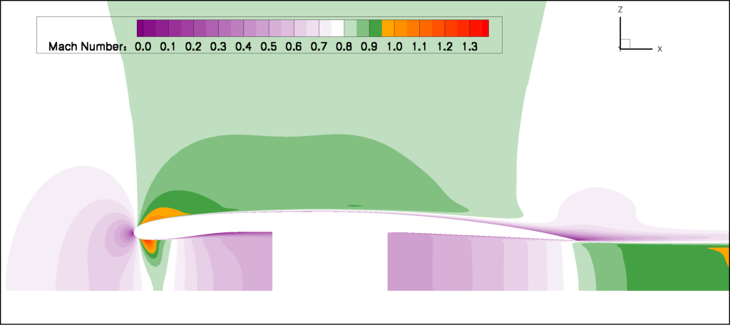
Mach slice bc_power_1.258_E1.200
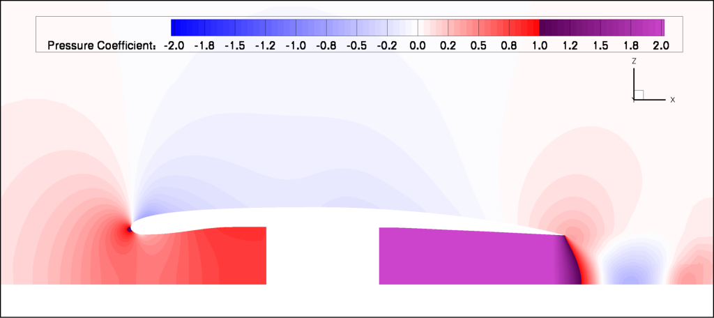
Cp slice bc_power_1.358_E2.000
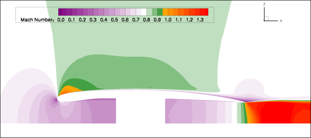
Mach slice bc_power_1.358_E2.000
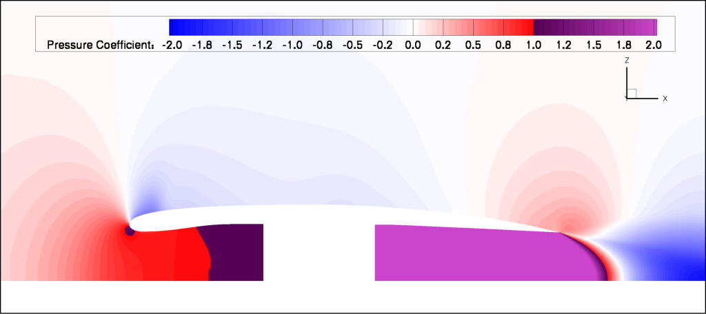
Cp slice bc_power_1.458_E4.000
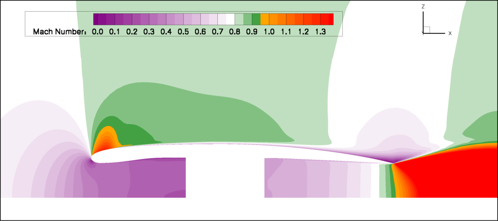
Mach slice bc_power_1.458_E4.000
