This pyOver example looks at the process from grid generation to execution and
post-processing for a simple bullet geometry. To start, clone the repo and
enter the resulting folder
the folder has the required input files, but it’s recommended to copy them to a
working folder so that it’s easy to reset. Just run the following command:
$ ./copy_files.py
$ cdwork/
This section guides the user through generating a grid system using Chimera
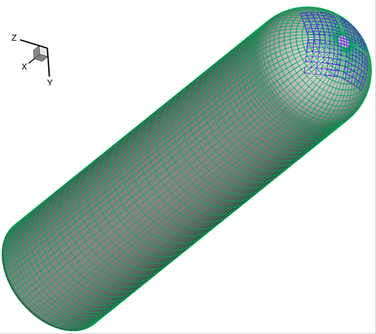
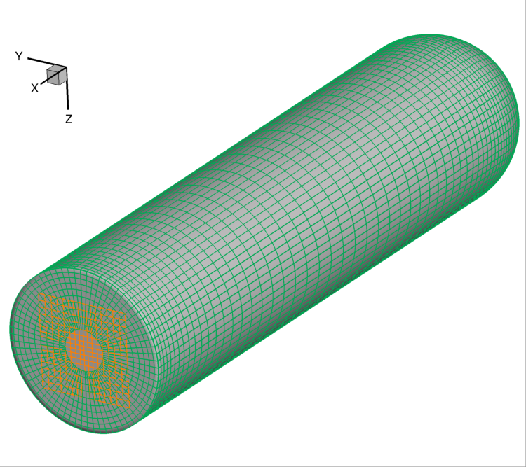
Grid Tools. The resulting surface grid system is shown in
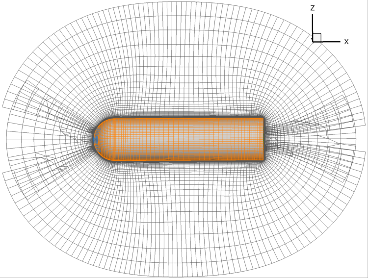
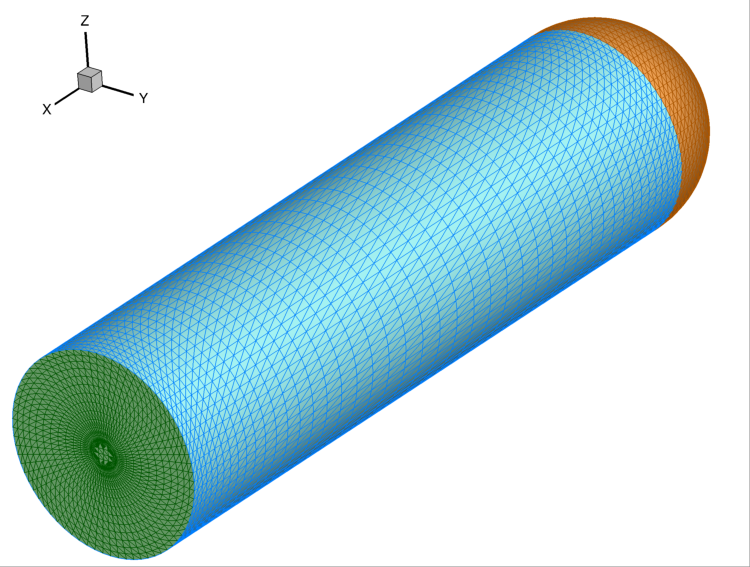
Table 6.1, and one view of the volume grid is shown in
Figure 6.1.
Table 6.1 OVERFLOW surface grid for bullet example
Front and side view
Aft view
Figure 6.1 OVERFLOW volume grid slice for bullet example
This is a three-grid system that demonstrates a lot of the basic features of
running OVERFLOW and creating a simple grid system.
While many users are opting to create overset grid systems using a graphical
user interface (for example Pointwise), this example guides users through a
traditional script-based grid generation process. While there are really no
special contributions of pyOver to this process, it may increase understanding
of later tasks to explain how the grid system was generated.
Some aspects of the grid generation example may rely on recent features of
Chimera Grid Tools.
Starting from the base directory for the example,
pyover01-bullet/, the grid generation takes place in the
dcf/ folder. The initial contents of this folder include a geom/
folder that contains the basic definitions for the geometry and some TCL
scripts for generating the grid.
dcf/
GlobalDefs.tcl: script to set overall variables for grid system
inputs.tcl: various local variables such as grid spacing
config.tcl: instructions for names of grids
geom/: geometry definitions folder
bullet.i.tri: surface geometry triangulation
bullet.stp: STEP file of relevant curves
bullet.lr8.crv: little-endian curve of axisymmetric radius
bullet/: grid building are for bullet component
BuildBullet.tcl: main script to generate bullet grids
localinputs.tcl: local settings for bullet component
Makefile: make instructions for building surface grids
The contents of the dcf/ directory are detailed above, but some aspects of
the TCL scripts are explained here. This example has only a single logical
“component,” called bullet, but a more general use case for the Chimera
Grid Tools grid script system may have many such components. For example, if
we added fins to this example, we may create the grids for those fins using
another folder called fins/.
Grid scripts rely on several hard-coded TCL file names, which can be guessed
from the layout of this dcf/ example. The GlobalDefs.tcl script sets a
few global variables for the grid script. None of the variables set in this
file are universal requirements, but those that are set in this TCL script can
become available to all of the other scripts. The contents of this particular
example of the GlobalDefs.tcl are shown below.
#!/usr/bin/env tclshglobalPar
# Source folder stuffsetScriptFile[filenormalize[infoscript]]setScriptDir[filedirname$ScriptFile]setRootDir[filejoin{*}[lrange[filesplit$ScriptDir]0end]]setGeomDir[filejoin$RootDirgeom]setPar(ScriptFile)$ScriptFilesetPar(ScriptDir)$ScriptDirsetPar(GeomDir)$GeomDir# Global switch for OVERFLOW solversetovfi_inputs"ssor"# List of parts includedsetIncludeBullet1# Grid scaling parametersetGlobalScaleFactor1.0
Some of this unusual TCL syntax is just intended to save the absolute path to
various folders, including the one containing the script (ScriptDir and
RootDir in this example) and the input geometry files (GeomDir). The
GlobalScaleFactor can also be used to change the overall resolution of grid
as long as all the other spacing variables are programmed to change with
GlobalScaleFactor.
The inputs.tcl file is much longer but is also a script that basically just
sets variables for use elsewhere. It defines basic grid resolution settings
with syntax such as
# ------
# Wall spacing and stretching ratio
# ------
set Par(ds,wall) 0.001
set Par(sr,wall) 1.2
set Par(klayer) 3
# ------
# Surface stretching ratio
# ------
set Par(sr)      1.2
set Par(sr,slow) 1.1
# ------
# Main marching distance
# ------
set Par(md)              5.0
set Par(md,protub)       2.0
set Par(md,protub,small) 1.0
It is a common convention to use Par as the TCL variable that stores
parameters for grid spacing. The inputs.tcl script also contains default
volume grid options
# ------
# Default hypgen inputs
# ------
set Par(smu) 0.5
set default(zreg)  $Par(md)
set default(dz0)   $Par(ds,wall)
set default(dz1)   $Par(ds,glb)
set default(srmax) $Par(sr)
set default(ibcja) -10
set default(ibcjb) -10
set default(ibcka) -10
set default(ibckb) -10
set default(imeth) 2
The volume options (hypgen options) can be overridden for individual
surface grids as needed. In addition the syntax
# ------# Volume grids created by other means# ------setbullet_body(nomakevol)1
instructs the BuildVol command not to grow a volume grid for the grid named
bullet_body because that volume grid is already created during the
execution of BuildBullet.tcl.
Within inputs.tcl, there are also instructions for what settings to use in
the template OVERFLOW namelist, overflow.inp:
# ------# Inputs for the OVERFLOW flow solver# ------setOvr(incore).T.
setOvr(nsteps)100setOvr(restrt).F.
setOvr(fmg).T.
setOvr(fmgcyc)"1000, 1000, 0"setOvr(nglvl)4setOvr(nfomo)2setOvr(dtphys)0.0setOvr(nitnwt)0setOvr(walldist)2
Of course, these can be altered later by cape.pyover using the
cape.pyover.overNamelist interface. Finally, the mixsurcomp variable can
be used to group surface families into larger components, which affects the
file mixsur.i that is built by BuildMixsuri.
The file config.tcl describes the list of grids to include (for each
component, in examples where that’s appropriate).
#!/usr/bin/env tclshsource[GetIfileGlobalDefs.tcl]source[GetIfileinputs.tcl]# List of bullet gridssetgrids"bullet/bullet_body bullet/bullet_cap bullet/bullet_base "# List of xrayssetxrays"bullet/bullet "# Convert variable namessetrootnames"$grids"setxraynames"$xrays"
This script is fairly self-explanatory for a simple example such as this, but
in more general cases this file often contains more logic for including or not
including grids based on component on/off switches in GlobalDefs.tcl. The
variables rootnames and xraynames are hard-coded and used by the grid
script system.
From the dcf/ folder, run the Chimera Grid Tools command
$ BuildSurf
However, users should take care to match endianness. The input file is
little-endian, so the one of the following system commands may be necessary.
Note that the csh versions of these commands would need to use setenv.
This command reads the rootnames variable and makes a list of all the folders
referenced by any grid, which in our simple example is simply bullet/.
Then the surface grid builder goes into each such folder and just calls
$ make
Therefore the contents of the Makefile in each component folder have a
direct impact. The contents for this Makefile are shown below. Basically
it instructs make to run the local script BuildBullet.tcl if any of
four files are missing or if any of two TCL files are newer than the grid
output files.
The other fixed-name file in the bullet/ folder is called
localinputs.tcl. This TCL script is sourced during the generation of
surface grids and of volume grids. The first part of this script sets spacings
and point counts specific to this component.
#!/usr/bin/env tclsh

global Ovr Par

# Body spacings
set Par(ds,bullet,cap)  [expr 0.10*$Par(ds,glb)]
set Par(ds,bullet,crn)  [expr 0.05*$Par(ds,glb)]
set Par(ds,bullet,body) [expr 0.25*$Par(ds,glb)]
set Par(ds,bullet,aft)  [expr 0.15*$Par(ds,glb)]

# Number of points around the bullet
set Par(npcirc,bullet) 73
Within the BuildBullet.tcl script contains many calls to the TCL utilities
of Chimera Grid Tools. After running this script (via BuildSurf or a
direct call) the following files are created in the bullet/ folder.
bullet_base.srf: surface grid bullet_base
bullet_body.srf: surface grid bullet_body
bullet_cap.srf: surface grid bullet_cap
bullet_body.vol: volume grid bullet_body
bullet_base.ovfi: OVERFLOW inputs for grid bullet_base
bullet_body.ovfi: OVERFLOW inputs for grid bullet_body
bullet_cap.ovfi: OVERFLOW inputs for grid bullet_body
bullet.xry: X-Ray cutter file for bullet’s body
These files demonstrate that one component may have multiple grids, and thus
the decision on what is a “component” and what is multiple components is
decided by the user for the specific situation. The grid script system keeps
all grid files separate (although to be clear these are multiple-grid format
with one grid).
Regarding the ovfi files, they contain namelists specifically for each
grid. These are assembled into the overflow.inp namelist for each included
grid (order is important).
Creating the volume grids is performed using the following system command, also
run from the dcf/ root folder.
$ BuildVol
This creates a volume grid for the two grids that did not have a previously
generated grid. The bullet_body.vol grid is generated by rotating a 2D
grid about the x-axis, so this volume does not need to be generated by
hypgen. After running BuildVol, the following additional files are
created.
To create the assembled volume and surface grids, the following (not
necessarily obvious) commands are run.
$ BuildPlot
This results in the surface grid file Composite.srf, which contains all
three surface grids combined into a single file.
$ BuildPlot-vol
This file creates Composite.vol, which is the primary volume grid that we
need as input to run OVERFLOW. Copy this file into the common/
subdirectory of the parent folder. The surface grid file is not required, but
can be convenient to have in a common location.
The following two commands create the template OVERFLOW input namelist and
mixsur input file, respectively.
$ BuildOveri
$ BuildMixsuri
After running the first command, the files overflow.inp and xrays.in
are created. Both of these files are also required for running, so they can be
copied into the ../common/ folder, too. However, the overflow.inp file
is already provided; users can compare them to check that they are identical.
$ cpxrays.in../common/
The BuildMixsuri command creates the file mixsur.i. We will need this
file later, first let’s apply the xrays by running OVERFLOW for zero
iterations. To run OVERFLOW in this manner, we set the namelist parameter
OMIGLB > IRUN to 2. The normal value is 0. Fortunately, the
overflow.inp file we created already has IRUN=2. Now we create a
folder called irun2/ and copy the necessary files into it. The following
commands can be run from the dcf/ folder.
Users who do not have a compiled MPI version of OVERFLOW can try .
$ overrunoverflow
This will run OVERFLOW and create quite a few output files. Most of these we
can ignore, but we will need x.save to run mixsur. In addition, for
more complex grids, this is the file that we inspect to see interpolation
quality and check the number of orphan points.
To run mixsur, let’s go up two folders and set things up to run mixsur
in the common/fomo/ folder. The term fomo is a common portmanteau for
“force and moment” in the OVERFLOW world.
The mixsur.i file is already in the fomo/ folder. Now we can enter
that folder and run mixsur.
$ cdcommon/fomo
$ mixsur<mixsur.i>mixsur.o
This creates a significant number of files, most of which are useful for at
least one OVERFLOW data analysis scenario. The file mixsur.fmp is critical
because it provides instructions to OVERFLOW on how to integrate the surface
pressures and viscous loads into component forces & moments. In addition, the
grid.i.tri file is a unique surface triangulation created from the surface
grid.
Figure 6.3 Surface tri from mixsur of OVERFLOW bullet surface grid
The surface triangulation created by mixsur is shown in
Figure 6.3. It shows that the surface has been divided
into three families, a cap, fuselage, and base, and that these do not
correspond to the boundaries between grids or something similar. These
boundaries are set within BuildBullet.tcl. In regions of overlapping
grids, mixsur picks a unique triangle (roughly the smallest available,
although this process becomes very complex in the general case) and then
creates “zipper” triangles to join together the triangles that are selected
from dividing the surface grid quads in half.
At this point, we have created all of the grid files that are needed, and we
are ready to start running OVERFLOW using pyOver.
In addition to the grid input files, overflow.inp template namelist, and
mixsur.fmp file all described in the previous section, the 01_bullet/
folder contains a master settings file pyOver.json and a run matrix
inputs/matrix.csv.
To run one case, we can run the following command. This will run the second
case in the matrix (index 1 according to Python’s 0-based indexing).
$ pyover-I1Case Config/Run Directory Status Iterations Que CPU Time---- --------------------- ------- ----------- --- --------1 poweroff/m0.8a4.0b0.0 --- / . Case name: 'poweroff/m0.8a4.0b0.0' (index 1) Starting case 'poweroff/m0.8a4.0b0.0' > overrunmpi -np 6 run 01 (PWD = '/examples/pyover/01_bullet/poweroff/m0.8a4.0b0.0') (STDOUT = 'overrun.out') Wall time used: 0.07 hrs (phase 0) Wall time used: 0.07 hrs Previous phase: 0.07 hrs > overrunmpi -np 6 run 02 (PWD = '/examples/pyover/01_bullet/poweroff/m0.8a4.0b0.0') (STDOUT = 'overrun.out') Wall time used: 0.08 hrs (phase 1) Wall time used: 0.14 hrs Previous phase: 0.08 hrs > overrunmpi -np 6 run 03 (PWD = /examples/pyover/01_bullet/poweroff/m0.8a4.0b0.0') (STDOUT = 'overrun.out') Wall time used: 0.05 hrs (phase 2)Submitted or ran 1 job(s).---=1,
As we can see, this ran OVERFLOW locally (i.e. without submitting a PBS job or
similar) using the MPI version and 6 processors (cores). The actions that
pyOver takes are fairly simple.
Create the poweroff/m0.8a4.0b0.0/ folder
Copy the requisite files into that folder
Run overrunmpi-np6run01
Run overrunmpi-np6run02
Run overrunmpi-np6run03
The basic JSON inputs that caused these actions to be taken are highlighted
below.
// Options for overall run control and command-line inputs"RunControl":{// Run sequence"PhaseSequence":[0,1,2],"PhaseIters":[1500,2000,2500],// Operation modes"Prefix":"run","MPI":true,"qsub":false,"mpicmd":null,"nProc":6,// OVERFLOW command-line interface"overrun":{"cmd":"overrunmpi","aux":null}}
As with any of the solver-specific cape modules, the PhaseSequence and
PhaseIters specify how many times and for how long the code is run. Here we
have phases 0, 1, and 2, which become runs 01, 02, and
03 for OVERFLOW (specifically overrunmpi). These phases are run until
there are 1500, 2000, and 2500 total global iterations run, respectively.
Setting MPI to true instructs pyOver to use an MPI version of OVERFLOW,
but setting mpicmd to null handles the special situation for
overrunmpi. The command-line calls to run OVERFLOW are handled by the
overrun section, and since we have the command set to "overrunmpi",
command-line calls do not start with mpiexec-np6... the way that most
MPI calls are. The executable overrunmpi is a script that calls
mpiexec internally, so we eliminate this prefix for the command called by
pyOver.
The actual number of iterations in one run of each phase is not set in the
RunControl section above. Instead, it is set within the overflow.inp
namelist using the setting GLOBAL>NSTEPS. Here we have 500 “steps”
(iterations) for each phase, but one run of phase 0 actually ends with 1500
iterations because this is NSTEPS[0]+FMGCYC[0][0]+FMGCYC[0][1]. We are
requesting three levels of multigrid cycles on phase 0, so we add those cycles
to the global iteration count.
Noe that the double list input for FMGCYC is important here because
"FMGCYC":[500,500] would be interpreted as 500 for phase 0 and
500 for all following phases. We actually need this to be a list so
[[500,500]] is interpreted as [500,500] for all phases.
We have to set OMIGLB>*IRUN* to 0 here so that OVERFLOW is actually run
for more than 0 iterations. The rest of the OMIGLB section sets mesh
adaptation inputs. The Grids top-level section of pyOver.json sets the
CFL number for each grid and other key OVERFLOW input settings. Below we have
the Mesh section, which instructs pyOver which files to copy (or link) into
each case folder.
// Mesh"Mesh":{// Folder containing definition files"ConfigDir":"common",// Grid type, dcf or peg5"Type":"dcf",// List or dictionary of files to link"LinkFiles":["grid.in","xrays.in","fomo/grid.ibi","fomo/grid.nsf","fomo/grid.ptv"],// List of files to copy instead of linking"CopyFiles":["fomo/mixsur.fmp"]}
For example, if the case is poweroff/m0.80a4.0b0.0, this effectively runs
the following commands.
// RunMatrix description"RunMatrix":{// If a file is specified, and it exists, trajectory values will be// read from it. RunMatrix values can also be specified locally."File":"inputs/matrix.csv","Keys":["mach","alpha","beta"],// Copy the mesh"GroupMesh":true,// Configuration name [default]"GroupPrefix":"poweroff"}
This example just has Mach number, angle of attack, and angle of sideslip as
inputs. This means that the Reynolds number per inch and freestream static
temperature are whatever values are in the template common/overflow.inp
namelist. In this case they are
After running case 1 as shown above, we can enter the folder to see what
files are present. First, let’s set up case 2 and not run it. That way we
can compare the files before running and after.
$ pyover-I2--no-start
Case Config/Run Directory Status Iterations Que CPU Time---- --------------------- ------- ----------- --- --------2 poweroff/m0.9a0.0b0.0 --- / . Case name: 'poweroff/m0.9a0.0b0.0' (index 2)Set up 1 job(s) but did not start.---=1,
The --no-start flag has the effect of not starting the case (or submitting
a job, if the qsub option were true). The files in this folder are
described below.
case.json: JSON RunMatrix settings for this case
conditions.json: JSON file with values of pyOver run matrix keys
grid.ibi: surface grid I-blanks file
grid.in: main input volume grid (near-body)
grid.nsf: another mixsur grid file
grid.ptv: another mixsur grid file
mixsur.fmp: weights for each surface point’s contribution to F & M
run.01.inp: input namelist for phase 0
run.02.inp: input namelist for phase 1
run.03.inp: input namelist for phase 2
run_overflow.pbs: BASH script that can be executed or submitted
xrays.in: input file for DCF X-ray generation
If we look in the poweroff/m0.8a4.0b0.0 folder that was already run, we
have those files and the following additional ones:
brkset.restart: brick grid file for adaptive off-body grids
brkset.save: brick grid file for adaptive off-body grids
fomoco.out: iterative force & moment history from most recent run
grdwghts.restart: another adaptive off-body grid info file
grdwghts.save: another adaptive off-body grid info file
log.out: streamed output from overrunmpi
mixsur.save: most recently used version of mixsur.fmp
overrun.out: STDOUT from most recent run
pyover_start.dat: date and time of start of each run
pyover_time.dat: time used for each run completed
q.restart: primary volume grid solution file
q.save: primary volume grid solution file
resid.out: iterative residual history on each grid
rpmin.out: minimum density and pressure on each grid, iterative
run.01.1500: STDOUT/STDERR from run 01
run.01.2000: STDOUT/STDERR from run 02
run.01.2500: STDOUT/STDERR from run 03
run.fomoco: assembled force & moment history
run.log: assembled log file
run.resid: assembled residual history
run.rpmin: assembled minimum density and pressure history
run.timers: OVERFLOW timing information
run.turb: turbulence residual history
timers.out: most recent OVERFLOW timing information
turb.out: turbulence residuals from most recent run
x.restart: final volume grid file
x.save: final volume grid file
While a case is currently running there are also files such as fomoco.tmp
that accumulate the force & moment history or other iterative history only for
the currently running phase. When a run completes, these are moved into
fomoco.out and copied into run.fomoco.
This case is also set up to create a simple report with several iterative
history plots. The command is simple.
$ pyover--report-I1
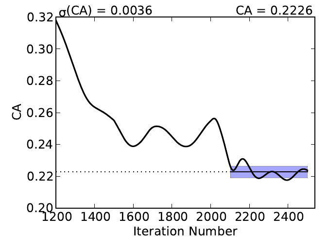
This generates two tables, one of which shows the values of input variables and
the other of which shows the iteratively averaged values and standard
deviations of CA, CY, and CN on three mixsur families.
Table 6.2 Sample iterative plots from OVERFLOW bullet case report for
poweroff/m0.8a4.0b0.0
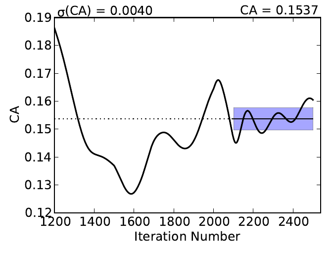
bullet/CA
cap/CA
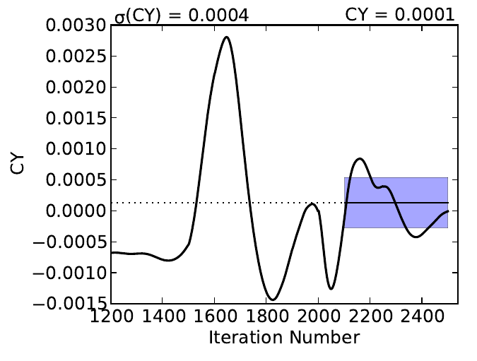
bullet/CY
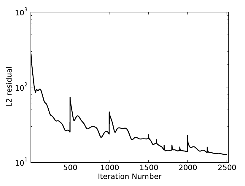
Global L2 residual
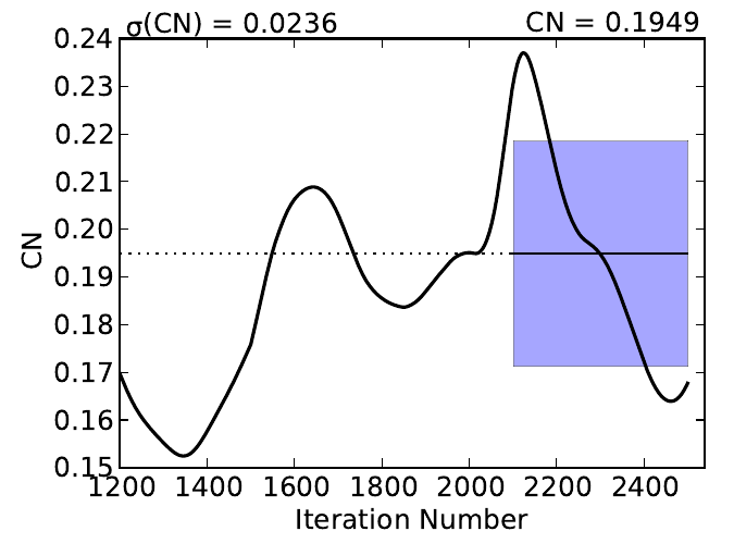
bullet/CN
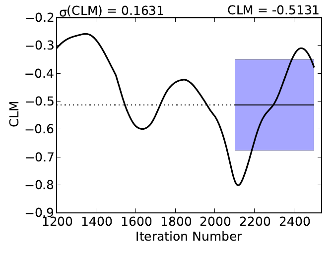
arrow/CLM
The averaging window for each coefficient is visible as a blue rectangle; the
width of the box is the iterative averaging window and the height is one
standard deviation above and below the mean value. The averaging window can
also be seen from where the dotted mean value horizontal line switches to a
solid line. The user can control the size of the iterative window (and give
pyOver some freedom to decide if a range of values is given) in the DataBook
section of pyOver.json using nStats and nStatsMax. The height of the
blue rectangle (as a multiple of the iterative standard deviation) is
controlled using the StandardDeviation parameter within each subfigure’s
definition in the Report section.
The plots in the previous subsection indicate that this case is not really
converged. To run the last phase another time, run the following simple
commands.
$ pyover-I1--extend
poweroff/m0.8a4.0b0.0 Phase 2: 2500 --> 3000$ pyover-I1Case Config/Run Directory Status Iterations Que CPU Time---- --------------------- ------- ----------- --- --------1 poweroff/m0.8a4.0b0.0 INCOMP 2500/3000 . 1.1 Starting case 'poweroff/m0.8a4.0b0.0' > overrunmpi -np 6 run 03 (PWD = '/examples/pyover/01_bullet/poweroff/m0.8a4.0b0.0') (STDOUT = 'overrun.out') Wall time used: 0.06 hrs (phase 2)Submitted or ran 1 job(s).INCOMP=1,
It is also possible to use a command like pyover-I1--extend2, which
would have instructed pyOver to run the last phase 2 more times, so we
would have had 3500 iterations overall.
Now we can check the overall status of the entire setup (four cases). We
should see something like the following.
$ pyover-c
Case Config/Run Directory Status Iterations Que CPU Time---- --------------------- ------- ----------- --- --------0 poweroff/m0.8a0.0b0.0 --- / .1 poweroff/m0.8a4.0b0.0 DONE 3000/3000 . 1.52 poweroff/m0.9a0.0b0.0 INCOMP 0/2500 .3 poweroff/m0.9a4.0b0.0 --- / .---=2, INCOMP=1, DONE=1,
On the system that was used 1.5 core hours; divide this by 6 to get the wall
time. Users can also rerun the pyover-I1--report command to get updated
iterative histories. The --report command is fairly intelligent about
deciding whether or not a figure needs to be updated when regenerating a
report.
Suppose instead of repeating the last phase we wanted to add another phase with
slightly different inputs. Then we can run very similar commands to above,
presumably after making sure that phase 3 has the new OVERFLOW inputs we
want in the pyOver.json file. It is also possible to add the --submit
flag at the end to combine the settings change and case restart commands.
$ pyover-I1--apply--submit
Keeping the distinction between --apply and --extend commands clear is
not always intuitive, but just remember that --apply has the property that
it is applying whatever settings are in the master JSON file to a case. This
command can be used to change other settings even if no additional phases are
being added, although of course this will not affect phases that have already
been run.
It is possible to get pyOver and its automated reports to coordinate
effectively with Tecplot®. The procedure is somewhat involved and can be
summarized as consisting of the following steps:
Enter a case folder with an appropriate solution and create a desirable
Tecplot layout manually
Save the layout file (.lay) to the inputs/ folder or somewhere
else accessible to pyOver
Modify that template layout file slightly for use with pyOver
Add the appropriate subfigure instructions to the Report section
Generate a report including the Tecplot-generated subfigure
Using Tecplot with OVERFLOW solutions is much more involved than solutions of
most other CFD solvers. Users reaching this region of the example may already
be experienced in generating Tecplot layouts, but this example includes a
reduced step-by-step procedure for generating the examples in this file.
First, go into the poweroff/m0.8a4.0b0.0 folder that contains our solution
files. Then launch Tecplot using whatever executable is set up on your system
and go to
File ‣ “Load Data…”.
Select “PLOT3D Loader” in the “Files of type” dropdown, and select and open
q.save and x.save.
This will open the solution but not draw any meaningful data yet. To find the
surfaces, click the “Zone Style…” button on the main left toolbar
and select the Surfaces tab. Select the first three zones, and then right
click in the “Surfaces to Plot” and select “K-Planes”. You can close the
“Zone Style…” window. This is a good time to use the menu option
View ‣ “Fit Surfaces…”
Next let’s calculate pressure coefficient (Cp) and local Mach number.
Fortunately this is already present in the
Analyze ‣ “Calculate Variables…”
Tecplot menu item. Press the Select… button in the window that opens, and
then select “Pressure Coefficient”, press Calculate, and repeat for “Mach
Number”.
Now we have to instruct Tecplot® to use the OVERFLOW I-blanks from our volume
grid file. (Why this is not the default is unclear.) Open the menu item
Next we instruct Tecplot® what to plot on the surface and what to plot on the
volume slice we will create. Check the Contour box on the main left toolbar
and press the Details… button. In the window that opens, click the
dropdown box in the top left and select “12: Pressure Coefficient”. We
should still be in the “Levels and Color” tab, and from there let’s press the
“Set Levels…” button.
This opens another window, and for this example let’s check the “Min, max and
delta” option from the “Range Distribution” box and make the following
selections:
“Minimum level”: -0.8
“Maximum level”: 0.8
“Detla”: 0.1
Press OK to close this window and then select “Diverging - Blue/Red” from the
dropdown box just below the “Color map options” label and interactive color
bar. Now let’s go to the Legend tab to tweak the legend and color bar drawn
on our figure. Make the following selections.
“Alignment”: Horizontal
“Level skip”: 2
“Size” (below “Number font”): 2
“Size” (below “Header font”): 2
Then click the “Legend Box…” and make the following selections:
Top option: select Fill
“Box color”: White
Close this window and click the “Number Format…” button about two thirds of
the way down the window. In the window that opens make the following
selections:
“Type”: Float
“Precision”: 1
After closing this window, we are still in the
“Contour & Multi-Coloring Details” window. Near the top of the window, click
on the 2 button. After clicking that, we set up the contour options for the
second contour plot, which is going to be the Mach number volume slice. After
clicking the 2, click on the top-left corner dropdown box and select
“13: Mach Number”. Then repeat all of the instructions above for the
Legend tab that we should currently still be in.
After repeating the Legend instructions, click again on the
“Levels and Color” tab and change the color map to
“Diverging - Purple/Green”. The “Set Levels..” button can also be modified
to the following settings:
“Range Distribution”: “Min, max, and delta”
“Minimum level”: 0
“Maximum level”: 1.6
“Delta”: 0.2
Finally we are finished with the contour details window. To get a nice fixed
view if the solution, click the Z-X button in the
“Snap to orientation view” near the top of the main left toolbar. Then check
the box to the left of Slices about half way down this toolbar and click the
Details… button to its right. We are going to make selections in several
of the tabs of the window that opens, using the following outline.
Definition tab
“Slice location”: Y-Planes
Contour tab
“Show contours”: checked
“Flood by”: C2: Mach Number
Other tab
“Show mesh”: checked
“Color” (mesh): Cust 2 (lightest gray available)
“Line thickness (%)”: 0.05
Ok, now select tha arrow tool from the top toolbar and click and drag the color
bar legends to the top left and top right (or anywhere else that looks good).
Then move the main window around until the field of view is appropriate, and we
have created a good layout.
To get rid of the orange dashed boxes that may be visible, make sure
Options ‣ “Show Bounding Boxes for …”
is unchecked. Figures also look better after opening the
Frame ‣ “Edit Active Frame…”
window and unchecking “Show border”.
Finally we can select
File ‣ “Save Layout as…”
to save the layout file. Save the layout as bullet-mach.lay so that we can
customize it and apply to other OVERFLOW solutions.
We have to manually edit the layout file we just created, bullet-mach.lay
to make very slight changes to the text. The third line of this file contains
many settings in a big list of strings. One of these will end with x.save,
and another will end with q.save. Replace these two strings (including any
folder names or absolute paths that precede them) with x.pyover.p3d and
q.pyover.p3d, respectively.
These file names are automatically created by pyOver during the report
generation file using its own logic to determine what is the most recently
available grid and solution file.
At this point you can compare your edited layout file with the one provided in
the /examples/pyover/01_bullet/inputs/bullet-mach.lay file. They should be
quite close except for at least some minor differences in camera position. If
desired, users are encouraged to copy the layout just created to the
inputs/ folder, preferably to a different file name so that the original
layout is still available.
In the main pyOver.json file, we need to add another subfigure in the
Report section to use this new layout file. To make this work, add the
following content. Don’t delete entries that aren’t shown below, but do edit
or add as necessary to match the following.
"Report":{"bullet":{"Figures":["CaseTables","CasePlots","FlowViz"]},"Figures":{"FlowViz":{"Header":"Flow visualization","Alignment":"center","Subfigures":["MachSlice"]}},// Definitions for subfigures"Subfigures":{// Tecplot figure"MachSlice":{"Type":"Tecplot","Layout":"inputs/bullet-mach.lay","FigWidth":1024,"Width":0.48,"Caption":"Surface $C_p$ and $y=0$ Mach slice","FieldMap":[3,1000]}}}
Most of these inputs are relatively self-explanatory, but the FieldMap
entry (while not actually required for this example) is worth explaining. This
controls Tecplot’s understanding of the “Zone Style…” window that we used
in a preceding subsection. It setting a large number for the last entry in
FieldMap is very useful because the number of grids generated by OVERFLOW for
the off-body solution can change, especially for adaptive solutions. The first
entry is 3 here, which it already was because we told Tecplot® that the
first three grids have a surface at K=1. Changing this FieldMap can be
very useful when trying to use previously generated Tecplot® layouts for new
grid systems that have a different number of surface grids.
Now if we rerun
$ pyover-I1--report
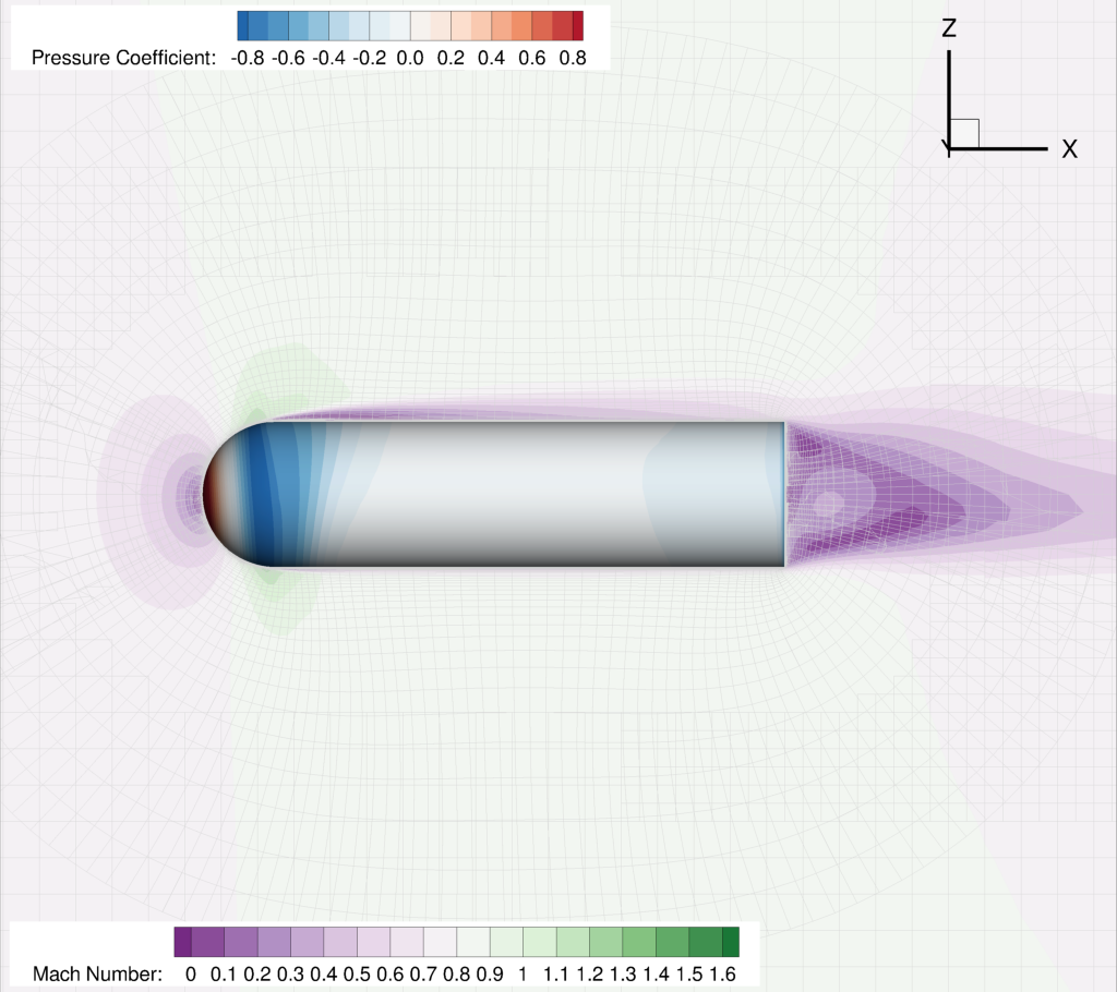
the automated report report/report-bullet.pdf will have a third page
containing an image like the one in Figure 6.4.
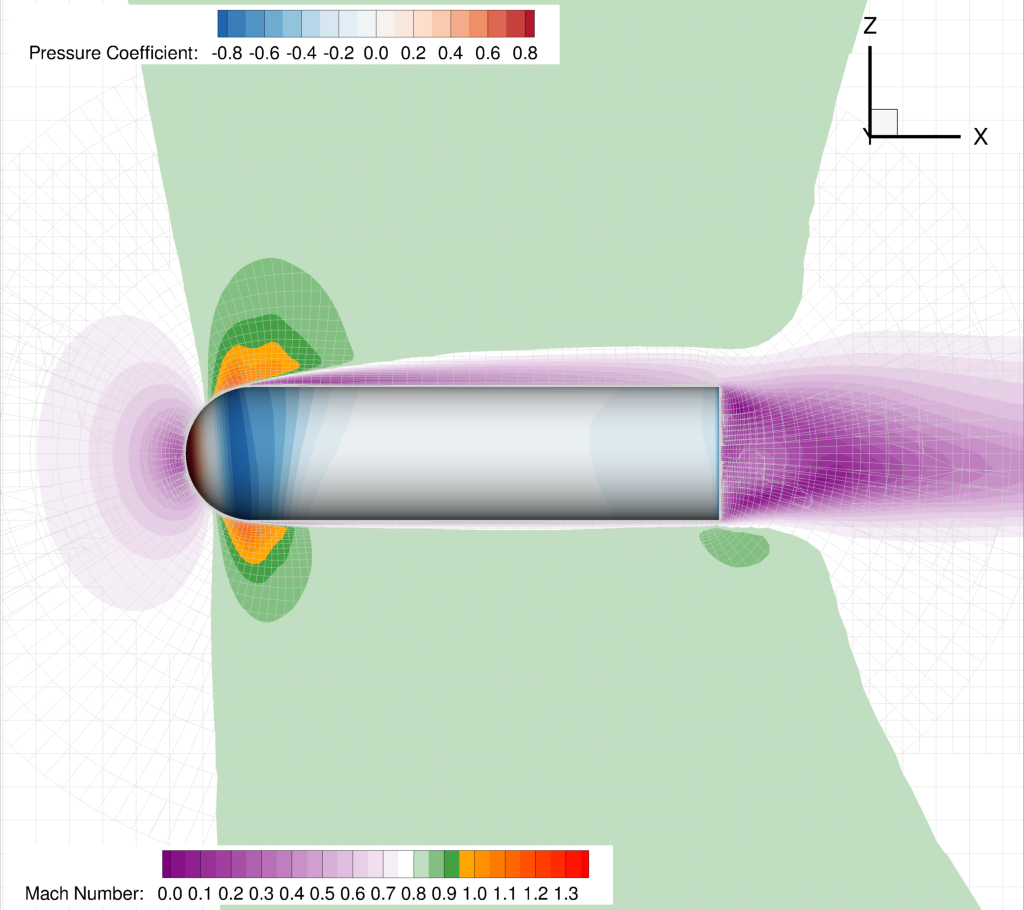
Figure 6.4 OVERFLOW bullet example MachSlice figure
This example does not take advantage of CAPE’s powerful capability to edit and
customize layouts on the fly. Let’s tweak the Mach number color map so that it
will alter the color map and also keep white exactly at the freestream Mach
number even if the Mach number changes. To do so, we will add another
subfigure called MachSlice-orange and base it off of what we just did.
"Report":{"Figures":{"FlowViz":{"Header":"Flow visualization","Alignment":"center","Subfigures":["MachSlice","MachSlice-orange"]}},// Definitions for subfigures"Subfigures":{"MachSlice-orange":{"Type":"MachSlice","ContourLevels":[{"NContour":2,"MinLevel":0,"MaxLevel":"max(1.4, 1.4*$mach)","Delta":0.05}],"ColorMaps":[{"Name":"Diverging - Purple/Green modified","NContour":2,"ColorMap":{"0.0":"purple","$mach":"white","1.0":["green","orange"],"max(1.4,1.4*$mach)":"red"}}],"Keys":{"GLOBALCONTOUR":{"LABELS":{"Parameter":2,"Value":{"AUTOLEVELSKIP":2,"NUMFORMAT":{"FORMATTING":"'FIXEDFLOAT'","PRECISION":1,"TIMEDATEFORMAT":"''"}}}}}}}}
Using Type=``”MachSlice”`` means that any settings not specified in this
subfigure are inherited from the MachSlice subfigure. We then set up the
Mach contour levels to be slightly finer and have an upper limit that depends
on the Mach number. In the ColorMaps parameter, we create a new color map
that has just a few control points, and some of those control points depend on
the run matrix variable. Using the syntax $mach in these control points
instructs pyOver to query the value from the run matrix. At the value
"1.0", i.e. Mach 1, we set two colors. This sets the first color
("green") as the lower bound and the second color ("orange") as the
upper bound; the result is a sharp boundary highlighting the sonic line.
This example is more complex than most applications because the Keys section
is needed to reduce the number of values printed in the legend for the Mach
number contour plot. The Mach contour plot is the second contour map in the
Tecplot layout, and really we’re just trying to change AUTOLEVELSKIP, but
since we never set one in our original layout, more instructions are needed.
This demonstrates how any layout command or variable can be edited, but usually
it’s easier to do this in the Tecplot® GUI.
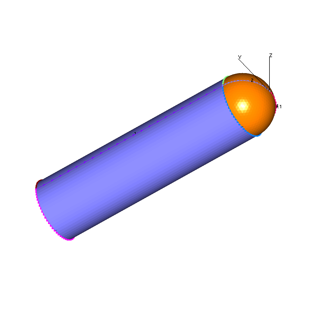
The result of this modified layout is shown in Figure 6.5.
Figure 6.5 OVERFLOW bullet MachSlice-orange flow viz with sonic line
The actual JSON file used to create these plots is saved as
pyOver-completed.json in the 01_bullet/ folder. Users may run the
other four cases and rerun the report command (pyover--report) to inspect
results for all four cases. Other modifications are encouraged, too, as this
is a fairly simple setup to extend and customize.