pg_example-batch.pro
batch filePG EXAMPLE
Created by Joe Spitale Edited by Mark Moretto for manual
This example demonstrates various capabilities of the PG programming interface, OMINAS' command-line API.
This example file can be executed from the shell prompt in the ominas/demo directory using:
 ominas pg_example-batch

or from within an OMINAS IDL session using:
@pg_example-batch
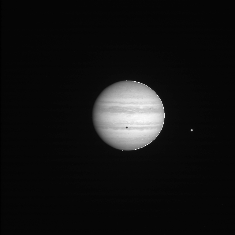
READ AND DISPLAY IMAGE
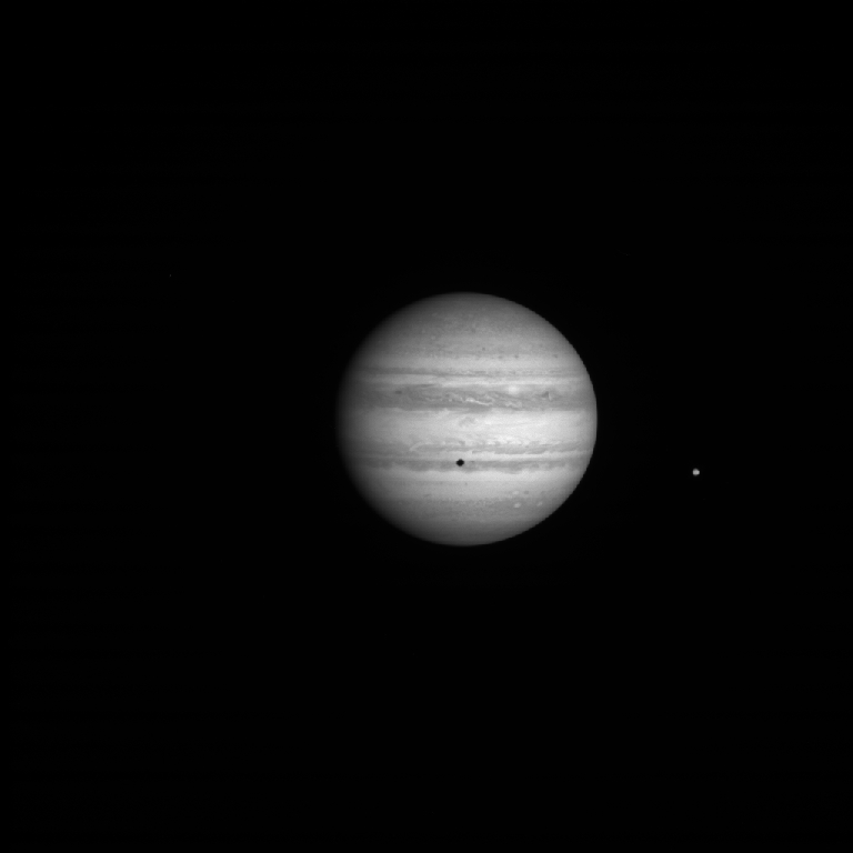
Use DAT_READ to read the image and then display the image using TVIM. With DAT_READ, it is not necessary to specify the file format. DAT_READ uses your file type detectors to determine the format, and gets the appropriate reader from your I/O table. DAT_READ returns a data descriptor (dd), which contains all of the data associated with the file. For convenience, it also returns the data array (im) and header (label) in its second and third arguments.
TVIM is called to display the image (im) in a new window with the y coordinate as top-down:
 dd = dat_read('./demo/data/N1350122987_2.IMG', im, label)
 tvim, im, zoom=0.75, /order, /new
OBTAIN GEOMETRY
This section obtains the geometric information describing the scene. Note that there is no reference to the source of the this information. That is handled by the translator system, which is controlled by a series of translators tables telling OMINAS which translators to use for a given instrument. The translators tables are parsed by DAT_READ, which stores the list of translators in the data descriptor.
If you are using the default demo configuration, then the geometry data are obtained via the NAIF/SPICE translator package and the detached header package. The NAIF/SPICE translators use database files provided by NAIF or by individual projects. The detached header translators read and write geometry descriptors in a text-based file that resides in the same directory as the data file and has the extension '.dh'. Because the detached header translator dh_std_input appears before the Cassini Spice input translator in the default translators table, the descriptors are taken from the detached header if it exists, and if the relevant descriptors are present. Otherwise, they are obtained from the SPICE kernels:
 cd = pg_get_cameras(dd)                        ; CAMERA descriptor
 pd = pg_get_planets(dd, od=cd, count=npd)      ; PLANET descriptor(s)
 rd = pg_get_rings(dd, pd=pd, od=cd, count=nrd) ; RING descriptor(s)
 ltd = pg_get_stars(dd, od=cd, name='SUN')     ; STAR descriptor for Sun
 pd = pg_get_planets(dd, od=cd, $
          name=['JUPITER', 'IO', 'EUROPA', 'GANYMEDE', 'CALLISTO'])
ii = where(cor_name(pd) EQ 'JUPITER')
INSTRUMENT-SPECIFIC USAGE
It is possible to communicate directly with the translators from the PG API via the use of translator keywords. Translator keywords are keyword=value strings that are passed directly to the translator system with no interpretation by OMINAS. They may be permanently coded in the translators table to be passed to a specific translator, or transient inputs may be provided to the PG_GET_* programs as a string argument. In the latter case, they are accessible to all translators pertaining to that PG_GET_* program and they precede translator keywords from the translators table.
Here are some examples of controlling the NAIF/SPICE interface in a call to PG_GET_CAMERAS:
 cd = pg_get_cameras(dd, 'klist=my_klist.txt')     ; Use personal kernel
                                                   ; list file.

 cd = pg_get_cameras(dd, 'ck_in=./test.bc')        ; Use a specified C kernel.

 cd = pg_get_cameras(dd, 'ck_in=./auto')           ; Use the C-kernel auto-
                                                   ; detect function.

 cd = pg_get_cameras(dd, 'klist=my_klist.txt, $    ; Multiple arguments
                          ck_in=test.bc;test1.bc') ; separated by commas;
                                                   ; multiple elements
                                                   ; separated by semicolons.
MAKE A GENERIC DESCRIPTOR
Here we go with the generic descriptors again. The story with these things is that long ago before GRIM was summoned from the lowest levels of heck, OMINAS (or MINAS, or NV) was purely command-based. That's what you want because you can always build a GUI on top of it, but it doesn't really work to start with a graphical tool and try to build a command-based system out of that. Therefore, I decided to have mercy on the poor jerks (mostly me up to now) who had to type (really paste) all of this nonsense in. The generic descriptor was therefore spawned as a way to cut down on all the cd=this, pd=that, bx=whatever that tends to go on. So we just shove it all into one structure and all of the PG programs know to look in there if one is given. Any explicit descriptor arguments take precedence, though. So if these things make you happy, then you're welcome. I rarely use them in this way. They live on because it turns out they have amazing utility in other ways. So anyway, it's like this:
gd = {cd:cd, gbx:pd, dkx:rd, ltd:ltd}
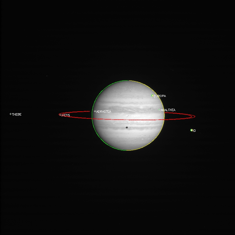
COMPUTE OVERLAY ARRAYS
These commands compute the center, limb, and terminator of each planet, as well as the edges of the rings. Note that the terminator is computed using PG_LIMB with the Sun as the observer:
 limb_ptd = pg_limb(gd=gd) & pg_hide, limb_ptd, gd=gd, bx=rd, /rm
           pg_hide, limb_ptd, /assoc, gd=gd, bx=pd, od=ltd
 ring_ptd = pg_disk(gd=gd) & pg_hide, ring_ptd, gd=gd, bx=pd
 term_ptd = pg_limb(gd=gd, od=gd.ltd) & pg_hide, term_ptd, gd=gd, bx=pd, /assoc
 center_ptd = pg_center(gd=gd, bx=pd)
SET UP FOR PLOTTING
This just makes the calls to PG_DRAW a little easier, since they will need to be repeated every time we change things and recompute. We put all of the POINT descriptors in one array and then make corresponding arrays for the plot parameters:
 object_ptd = [center_ptd,limb_ptd,ring_ptd,term_ptd]
 colors=[make_array(npd,value=!p.color), $
         make_array(npd,value=ctyellow()), $
         make_array(2*nrd,value=ctred()), $
         make_array(npd,value=ctgreen())]
 psyms=[make_array(npd,value=1), $
        make_array(npd,value=3), $
        make_array(2*nrd,value=3), $
        make_array(npd,value=3)]
 psizes=1.0
 csizes=0.75
 plabels=[cor_name(pd), $
         make_array(npd,value=''), $
         make_array(2*nrd,value=''), $
         make_array(npd,value='')]
DRAW EVERYTHING
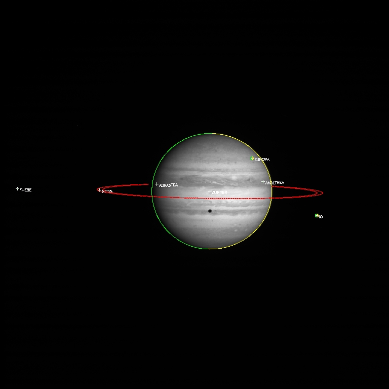
Now we can do a nice simple call to PG_DRAW to draw everything:
   pg_draw, object_ptd, $
             col=colors, psy=psyms, psi=psizes, csi=csizes, pl=plabels
FIRST-CUT AUTOMATIC REPOINTING
Refine the pointing of the spacecraft by using PG_FARFIT, which searches the image for a pattern matching the edges calculated using the geometry descriptors. First scan the images for edges, ignoring the a 10-pixel zone at the edge of the image:
 edge_ptd = pg_edges(dd, edge=10)
 pg_draw, edge_ptd
Next, use PG_FARFIT to find the x/y offset that best matches the limb of Jupiter (planet index ii):
dxy = pg_farfit(dd, edge_ptd, [limb_ptd[ii]])
pg_repoint, dxy, gd=gd
limb_ptd = pg_limb(gd=gd) & pg_hide, limb_ptd, gd=gd, bx=rd, /rm
       pg_hide, limb_ptd, /assoc, gd=gd, bx=pd, od=ltd
ring_ptd = pg_disk(gd=gd) & pg_hide, ring_ptd, gd=gd, bx=pd
center_ptd = pg_center(gd=gd, bx=pd)
term_ptd = pg_limb(gd=gd, od=gd.ltd) & pg_hide, term_ptd, gd=gd, bx=pd, /assoc
object_ptd = [center_ptd,limb_ptd,ring_ptd,term_ptd]
tvim, im pg_draw, object_ptd, $ colors=colors, psyms=psyms, psizes=psizes, plabel=plabels
MANUALLY REPOINT THE GEOMETRY
If you have a little time, you can just drag the pointing around by hand. We just need to get it close enough to really nail down in the next section. There's a good chance PG_FARFIT really dropped the ball on the last step anyway. Just paste this in and follow the directions:
tvim, im
dxy = pg_drag(object_ptd, dtheta=dtheta, axis=center_ptd[ii])
pg_repoint, dxy, dtheta, axis=center_ptd[ii], gd=gd
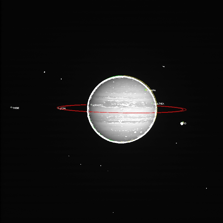
PRECISE EDGE SCAN
Not satisfied with PG_FARFIT? I wouldn't be, it's just not a sub-pixel kind of thing. Sometimes its results can be very super-pixel. However, once we get within a few tens of pixels of the correct pointing, we can use PG_CVSCAN to pick up the edges with a more rigorous algorithm. PG_CVSCAN scans around a predicted edge (in this case Jupiter's limb) comparing the brightness profile with a model profile. In this case, we use the limb edge model developed by Gary Yagi and used in the old VICAR NAV program (Ugh, remember VICAR? That's kind of the whole reason we're doing any of this). Indeed this whole CVSCAN business is the same exact algorithm that Andy Ingersoll scribbled down on a piece of paper sometime in the 1980s, just gussied up and vectorized with a bunch of pg_this and gd_that and all manner of other whatnot.
Anyway, here we are staying 30 pixels from the image edge, and scanning with a width of 80 pixels. lzero and mzero are coordinating the zero pointing of the model:
cvscan_ptd=pg_cvscan(dd, gd=gd, limb_ptd[ii], edge=30, width=80, $
   model=[make_array(npd,val=ptr_new(edge_model_nav_limb(zero=lzero)))], $
   mzero=[make_array(npd,val=lzero)] )
tvim, im
pg_draw, cvscan_ptd
THRESHOLD ON CORRELATION COEFFICIENT
This section calls pg_threshold to remove points with unacceptable correlation coefficients. The /relative flag means that the minimum and maximum thresholds are taken as a fraction of the maximum correlation coefficient for each set of points. In this case we use a minimum correlation coefficient of 0.81 and a maximum of 1.0:
 pg_threshold, cvscan_ptd, min=0.81, max=1.0, /rel
 tvim, im
 pg_draw, cvscan_ptd
MANUALLY EDIT THE SCANNED POINTS
PG_SELECT is used to manually remove points within a polygonal region defined by the cursor. PG_TRIM removes the points in the defined region:
 region = pg_select(dd)
 pg_trim, dd, cvscan_ptd, region
 tvim, im
 pg_draw, cvscan_ptd
SUB-PIXEL POINTING CORRECTION
PG_CVSCAN_COEFF determines the linear least-squares coefficients for a fit to the image coordinate translation and rotation that matches the computed curve to the scanned curve. PG_FIT uses the resulting coefficients to calculate the corrections. In this case, we fix the rotation offset (fix=2) because the limb gives little leverage on that parameter:
cvscan_cf = pg_cvscan_coeff(cvscan_ptd, fix=2)
dxy = pg_fit(cvscan_cf)
Once again, you need to recompute and redraw to see the new pointing:
FIT STATISTICS
You can get the statistics using PG_CHISQ and PG_COVARIANCE:
chisq = pg_chisq(dxy, 0, cvscan_ptd, fix=2)
covar = pg_covariance(cvscan_cf)
print, dxy, dtheta*180./!pi, chisq, covar
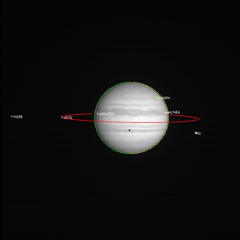
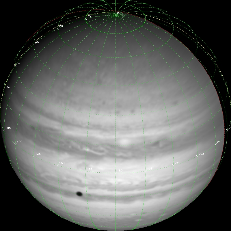
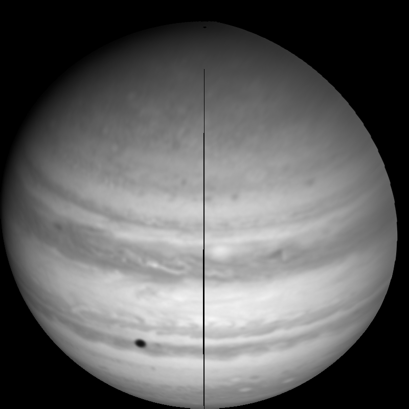
PLANET AND RING LATITUDE/LONGITUDE GRID
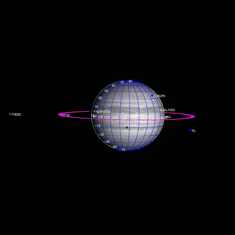
This section calculates a latitude/longitude grid for each planet and a radius/longitude grid for the rings. By default it draws 12 latitude and 12 longitude grid lines. The longitude grid lines circle the body and so on a map they will appear as 24 grid lines. The ring radius grid uses four grid lines by default between the inner and outer ring radius. It uses PG_HIDE to set as not visible the points on the grid behind the planet and ring for both objects. It then uses PG_DRAW to draw the grid points in blue (ctblue):
 grid_ptd = pg_grid(gd=gd, lat=lat, lon=lon)
 pg_hide, grid_ptd, cd=cd, bx=pd, /assoc
 pg_hide, grid_ptd, cd=cd, bx=pd, od=ltd, /assoc
 pg_hide, grid_ptd, gd=gd, bx=rd
 pg_draw, grid_ptd, color=ctblue()

 plat_ptd = pg_grid(gd=gd, slon=!dpi/2d, lat=lat, nlon=0)
 pg_hide, plat_ptd[ii], cd=cd, bx=pd[ii], /, bx=pd
 pg_draw, plat_ptd[ii], psym=3, plabel=strtrim(round(lat*180d/!dpi),2), /label_p

 plon_ptd = pg_grid(gd=gd, slat=0d, lon=lon, nlat=0)
 pg_hide, plon_ptd[ii], cd=cd, bx=pd[ii], /assoc
 pg_draw, plon_ptd[ii], psym=3, plabel=strtrim(round(lon*180d/!dpi),2), /label_p

 dgrid_ptd=pg_grid(gd=gd, bx=rd) & pg_hide, dgrid_ptd, gd=gd, bx=pd
 pg_draw, dgrid_ptd, color=ctpurple()
MAP DESCRIPTORS
PG_GET_MAPS is used to define map descriptors for various projections. Paste the one you want:
Rectangular:
 md = pg_get_maps(/over, bx=pd[ii], $
        projection='RECTANGULAR', $
        /map_graphic,
        size=[400,200])
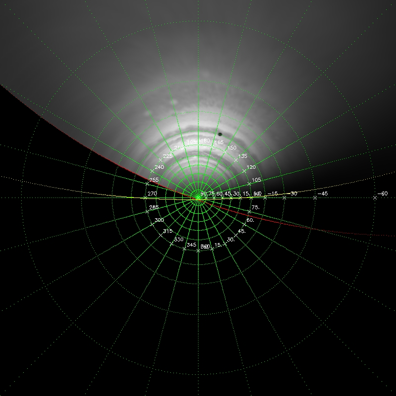
Orthographic:
  md = pg_get_maps(/over, bx=pd[ii], $
        projection='ORTHOGRAPHIC', $
        size=[400,400], $
        center=[!dpi/6d,!dpi])
Stereographic:
  md = pg_get_maps(/over, bx=pd[ii], $
         projection='STEREOGRAPHIC', $
         scale=0.5, $
         size=[400,400], center=[!dpi/2d,0d])
Mercator:
  md = pg_get_maps(/over, bx=pd[ii], $
        projection='MERCATOR', $
         size=[400,200])
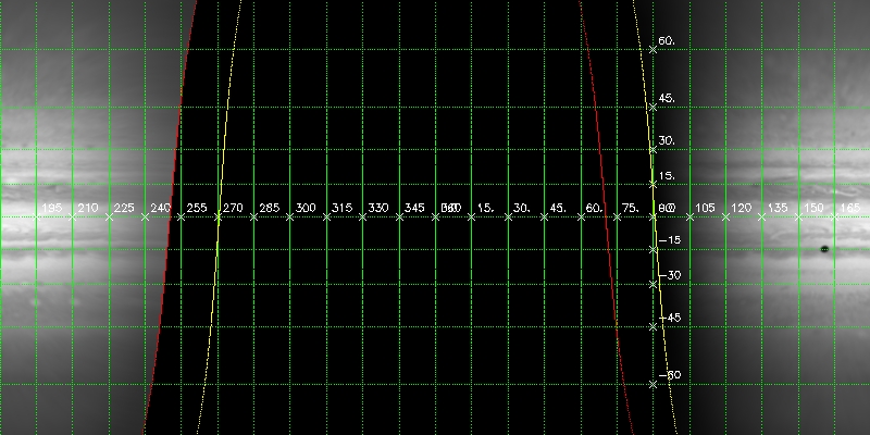
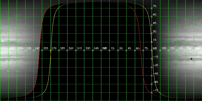
MAP PROJECTIONS
PG_MAP creates a map projection and returns it in a data descriptor. The map is also returned a a keyword for convenience:
 dd_map = pg_map(dd, md=md, gd=gd, bx=pd[ii], map=map)
 tvim, /new, map
 dd_map = pg_map(dd, md=md, gd=gd, bx=pd[ii], map=map, $
                  bounds=bounds = [-30,30,-180,180]*!dpi/180d)
 dd_map = pg_map(dd, md=md, gd=gd, bx=pd[ii], gbx=pd[ii], $
                    hide_fn='pm_hide_ring', hide_bx=rd, map=map)
PUT A GRID ON IT
PG_GRID computes a latitude/longitude grid. This is the same program used in other examples to draw grids on other things; here we're using a map descriptor instead of a camera descriptor.
First, define a new generic descriptor. :
 gdm={cd:md, od:cd, gbx:pd[ii], dkx:rd}

 map_grid_ptd = pg_grid(gd=gdm, lat=lat, lon=lon)
 plat_ptd = pg_grid(gd=gdm, slon=!dpi/2d, lat=lat, nlon=0)
 plon_ptd = pg_grid(gd=gdm, slat=0d, lon=lon, nlat=0)

 pg_draw, map_grid_ptd, col=ctgreen()
 pg_draw, plat_ptd, psym=7, plabel=strmid(strtrim(lat*180d/!dpi,2),0,3), /label_p
 pg_draw, plon_ptd, psym=7, plabel=strmid(strtrim(lon*180d/!dpi,2),0,3), /label_p
OBSERVATION-SPECIFIC OVERLAYS
Use PG_LIMB to compute a limb and a terminator by specifying an observer descriptor:
map_limb_ptd = pg_limb(gd=gdm, od=cd)
map_term_ptd = pg_limb(gd=gdm, od=ltd)

pg_draw, map_limb_ptd, col=ctred()
pg_draw, map_term_ptd, col=ctyellow()
MAP-TO-MAP PROJECTION
A map can be reprojected using a second map descriptor with the original map descriptor in place of the camera descriptor:
 md1 = pg_get_maps(/over, bx=pd[ii], $
    projection='ORTHOGRAPHIC', $
    size=[400,400], $
    center=[!dpi/6d,!dpi])

 dd_map1 = pg_map(dd_map, md=md1, cd=md, map=map1)
 tvim, /new, map1
OUTPUT DESCRIPTORS
These commands write the descriptor information out through the translators. The exact behavior is translator-dependent. In the default configuration, the detached header translator modifies the detached header stored in the data descriptor. It is not written until DAT_WRITE is called. We write only pd[0] because some translator setups may return large numbers of planet descriptors, making it pretty slow:
 pg_put_rings, dd, od=cd, rd=rd
 pg_put_planets, dd, od=cd, pd=pd[0]
 pg_put_cameras, dd, cd=cd
 pg_put_stars, dd, sd=ltd, od=cd
print, transpose(dat_dh(dd))
 cor_set_udata, cd, 'CK_COMMENT', 'This is a comment.'
 pg_put_cameras, dd, cd=cd, 'ck_out=./outputs/test.bc'
WRITE DATA FILE
DAT_WRITE writes the data array in the data descriptor using whatever output function was given in the I/O table. The detached header is is also written into a file with the same name as the image file except with the extension '.dh'. If this file does not already exist, it is created:
dat_write, './outputs/' + cor_name(dd), dd
WRITE MAP FILE
PG_PUT_MAPS causes the detached header translator to generate a new detached header and write the map descriptor into it.
As above, DAT_WRITE writes the map image file and the detached header. Notice that the file type is given explicitly because the data descriptor was not created by DAT_READ, which would have detected the file type:
 pg_put_maps, dd_map, md=md
 dat_write, './outputs/' + cor_name(dd) + '.map', dd_map, filetype = 'VICAR'
 dd_map = dat_read(./outputs/<nme>.map', map)
 md = pg_get_maps(dd_map)
 tvim, /new, map
File attributes
| Modification date: | Mon Jan 7 14:49:55 2019 |
| Lines: | 135 |
| Docformat: | rst rst |