Hazard Extraction and Analysis of Trends (HEAT): SAFECOM
This notebook provides an example of the trend analysis portion of the Hazard Extraction and Analysis of Trends framework. Trend analysis is applied the the SAFECOM dataset of wildfire aviation mishaps, available here: https://www.safecom.gov/
This example uses the trend analysis module from MIKA’s knowledge discovery toolkit, as well as the Data utility and SAFECOM utilities.
Prior to this analysis, hazard extraction is performed using the topic model plus module.
Imports
[1]:
import pandas as pd
import numpy as np
%matplotlib inline
import matplotlib.style
matplotlib.style.use("seaborn-v0_8")
import matplotlib.pyplot as plt
import matplotlib.cm as cm
import textwrap
import seaborn as sn
sn.color_palette("hls", 17)
import scipy.stats as st
import math
from sklearn.metrics import cohen_kappa_score
import pingouin as pg
plt.rcParams["font.family"] = "Times New Roman"
[2]:
import sys
import os
sys.path.append(os.path.join("..", "..", "..", ".."))

from mika.kd.trend_analysis import *
from mika.utils import Data
from mika.utils.SAFECOM import *
SAFECOM Data
Prior to performing HEAT, the SAFECOM dataset needs to be loaded in and cleaned.
The MIKA Data class is used for loading in the preprocessed data.
Additional cleaning includes: - identifying event occurrence year - removing non-fire reports - correcting regions
[3]:
list_of_attributes = ['Narrative']
extra_cols = ['Agency', 'Region', 'Location', 'Date', 'Date Submitted', 'Tracking #',
              'Mission Type', 'Persons Onboard', 'Departure Point', 'Destination',
              'Special Use', 'Damages', 'Injuries', 'Hazardous Materials', 'Other Mission Type',
              'Type', 'Manufacturer', 'Model', 'Hazard', 'Incident Management',
              'UAS', 'Accident', 'Airspace', 'Maintenance', 'Mishap Prevention'
              ]
document_id_col = 'Tracking #'

file = os.path.join('topic_model_results','preprocessed_data.csv')
safecom = Data()
safecom.load(file, preprocessed=True, id_col=document_id_col, text_columns=list_of_attributes)
preprocessed_df = safecom.data_df
[4]:
#extract event occurrence year
preprocessed_df['Year'] = [preprocessed_df.at[i,'Date'].split('/')[-1] for i in range(len(preprocessed_df))]
preprocessed_df['Day'] = [preprocessed_df.at[i,'Date'].split('/')[1] for i in range(len(preprocessed_df))]
preprocessed_df['Month'] = [preprocessed_df.at[i,'Date'].split('/')[0] for i in range(len(preprocessed_df))]
[5]:
preprocessed_df = preprocessed_df.loc[(preprocessed_df['Year'].astype(int)<2021) & (preprocessed_df['Year'].astype(int)>1994)].reset_index(drop=True)
[6]:
#remove ids from results file and preprocessed_df if the mission is non-fire
non_fire_missions = [mission for mission in list(preprocessed_df['Mission Type']) if type(mission) is str and 'non-fire' in mission.lower()]
ids_to_drop = preprocessed_df.loc[preprocessed_df['Mission Type'].isin(non_fire_missions)]['Tracking #'].tolist()
preprocessed_df = preprocessed_df.loc[~preprocessed_df['Tracking #'].isin(ids_to_drop)].reset_index(drop=True)
print(len(ids_to_drop))
1983
[7]:
#correct regions to match corresponding USFS regions
preprocessed_df = correct_regions(preprocessed_df)
[8]:
preprocessed_df
[8]:
| Agency | Region | Location | Date | Date Submitted | Tracking # | Mission Type | Persons Onboard | Departure Point | Destination | ... | UAS | Accident | Airspace | Maintenance | Mishap Prevention | Raw_Narrative | Year | Day | Month | region_corrected | |
|---|---|---|---|---|---|---|---|---|---|---|---|---|---|---|---|---|---|---|---|---|---|
| 0 | Bureau of Land Management (BLM) | Alaska State Office | Fairbanks | 05/10/1995 | 95-0002 | Fire, Smokejumper | 1.0 | Fairbanks | ... | Intrusion | On a practice parachute jump a single engine a... | 1995 | 10 | 05 | Region 10 Alaska Region | ||||||
| 1 | Bureau of Land Management (BLM) | Alaska State Office | Fort Wainwright | 05/10/1995 | 95-0003 | Fire, Smokejumper | 4.0 | Birch Hill | ... | Intrusion | NXXXXX 5-10-95 A small airplane flew thr... | 1995 | 10 | 05 | Region 10 Alaska Region | ||||||
| 2 | Bureau of Land Management (BLM) | Alaska State Office | Fort Wainwright | 05/09/1995 | 95-0004 | Fire, Air Attack | 2.0 | Fort Wainwright | ... | Electrical | After takeoff from Ft. Wainwight, left generat... | 1995 | 09 | 05 | Region 10 Alaska Region | ||||||
| 3 | Bureau of Land Management (BLM) | California State Office | BFL | 07/28/1995 | 95-0006 | Fire, Air Attack | 2.0 | BFL CA. | ... | Hydraulic | Firewall fitting cracked - leaking hydraulic f... | 1995 | 28 | 07 | Region 05 Pacific Southwest Region | ||||||
| 4 | Bureau of Land Management (BLM) | Alaska State Office | Fire B307 | 06/14/1995 | 95-0009 | Fire, Leadplane | 1.0 | Fire B307 | ... | Intrusion | While working fire B307 as a lead/air attack w... | 1995 | 14 | 06 | Region 10 Alaska Region | ||||||
| ... | ... | ... | ... | ... | ... | ... | ... | ... | ... | ... | ... | ... | ... | ... | ... | ... | ... | ... | ... | ... | ... |
| 12546 | Fish & Wildlife Service (FWS) | R4-Southeast Regional Office | Haines City | 11/18/2020 | 21-0138 | Fire, Other | 0.0 | Everglades Headwaters NWR Complex - Hatchineha... | Everglades Headwaters NWR Complex - Hatchineha... | ... | Fleet Operation, Loss of Link, Loss of GPS | The Parrot Anafi was flying an autonomous mapp... | 2020 | 18 | 11 | Region 08 Southern Area Region | |||||
| 12547 | State | California | McClellan Reload Base | 12/20/2020 | 21-0151 | Fire, Leadplane | 0.0 | ... | Prior to pilots' preflight, ATS noticed eviden... | 2020 | 20 | 12 | Region 05 Pacific Southwest Region | ||||||||
| 12548 | State | California | Hemet Airport | 12/24/2020 | 21-0152 | Fire, Retardant Drop (Airtanker) | 1.0 | KHMT | KRNM | ... | While fueling at Ramona AAB after 2.5 hour fue... | 2020 | 24 | 12 | Region 05 Pacific Southwest Region | ||||||
| 12549 | State | California | Camp Pendleton | 12/24/2020 | 21-0154 | Fire, Water Drop (Helicopter Fixed-Tank) | 3.0 | KCRQ | Creek Fire Camp Pendleton | ... | While engaged in a water dropping mission HT-7... | 2020 | 24 | 12 | Region 05 Pacific Southwest Region | ||||||
| 12550 | State | California | Chico Airport | 10/23/2020 | 21-0205 | Fire, Air Attack | 2.0 | Chico | Chico | ... | I was returning to Chico Airport from a fire d... | 2020 | 23 | 10 | Region 05 Pacific Southwest Region |
12551 rows × 30 columns
Hazard Extraction and Primary Analysis
First hazards are identified in documents using LDA topic modeling results and a hazard interptretation spreed sheet created from the topics.
The hazard file and LDA results file are specified here:
[9]:
hazard_file = os.path.join('topic_model_results', 'hazard_interpretation_SAFECOM_Final.xlsx')
results_file = os.path.join('topic_model_results','lda_results.xlsx')
Next, the hazard and results file are passed into the identify_docs_per_hazard function, which returns the frequency and documents associated with each hazard in addition to the hazard words and topics per each document:
[10]:
frequency, docs, hazard_words_per_doc, topics_per_doc, hazard_topics_per_doc = identify_docs_per_hazard(hazard_file, preprocessed_df, results_file, 'Raw_Narrative', 'Year', "Tracking #", 'Narrative', doc_topic_dist_field='document topic distribution', topic_thresh=0.0)#, ids_to_drop= ids_to_drop)
100%|██████████| 26/26 [04:05<00:00, 9.44s/it]
Then a severity fucntion is defined to calculate hazard severity. We define severity in this case using the function below:
[11]:
def safecom_severity(passengers, injury, damage):
    key_dict = {"No":0, "Yes":1}
    if passengers == '':
        passengers = 0
    severity = float(passengers)*(key_dict[injury] + key_dict[damage])
    if np.isnan(severity):
        severity=0
    return severity
Severity is calculated for each document using the defined function:
[12]:
preprocessed_df['severity'] = [safecom_severity(preprocessed_df.iloc[i]['Persons Onboard'], preprocessed_df.iloc[i]['Injuries'], preprocessed_df.iloc[i]['Damages']) for i in range(len(preprocessed_df))]
Now we create the primary results table. The category and subcategory for each hazard is identified from the documents using the get_categories_from_docs function. Finally, the table is created using the create_table function.
[13]:
hazards = frequency.keys()
categories, sub_categories = get_categories_from_docs(docs, preprocessed_df, "Tracking #")
categories = categories.values()
subcategories = sub_categories.values()
table, severities, rates = create_table(docs, frequency, preprocessed_df, "Tracking #", categories, subcategories, hazards, 'Year')
For display purposes, the table is re-indexed by hazard category and subcategory:
[14]:
table = table.sort_values(['Category', 'Subcategory'], axis=0).reset_index(drop=True)
df = table[['Category', 'Subcategory']]
ind = pd.MultiIndex.from_frame(df)
table.index = ind
table = table.drop(['Category', 'Subcategory'], axis=1)
The resulting primary results table:
[15]:
table
[15]:
| Hazards | Frequency | Rate | Severity | ||
|---|---|---|---|---|---|
| Category | Subcategory | ||||
| Airspace | Intrusion | Intrusion | 676 | 26.000 | 0.010 |
| Intrusion | Airspace Control Hazards | 732 | 28.154 | 0.078 | |
| Hazard | Communications | Radio Malfunction | 680 | 26.154 | 0.041 |
| Communications | Jumper Operations Hazards | 138 | 5.308 | 2.171 | |
| Mission Equipment | Prescribed Burn Operations Failure | 311 | 11.962 | 0.185 | |
| Other | Load Limits Exceeded | 193 | 7.423 | 0.144 | |
| Other | Cargo Letdown Failure | 626 | 24.077 | 0.280 | |
| Other | Door Failure | 413 | 15.885 | 0.404 | |
| Pilot Action | Water Drop Bucket or Tank Failure | 608 | 23.385 | 0.349 | |
| Pilot Action | In-flight Collision | 707 | 27.192 | 0.748 | |
| Policy Deviation | Inadequate PPE | 92 | 3.538 | 0.333 | |
| Policy Deviation | Personnel Duty Hours Exceeded | 225 | 8.654 | 0.102 | |
| Policy Deviation | Medivac | 143 | 5.500 | 2.178 | |
| Weather | Severe Weather | 499 | 19.192 | 0.449 | |
| Maintenance | Airframe | Structural Damage | 505 | 19.423 | 0.626 |
| Chip Light | On-board Caution Light Illuminates | 1809 | 69.577 | 0.109 | |
| Electrical | Avionics Malfunction | 214 | 8.231 | 0.148 | |
| Electrical | Electrical Failure | 727 | 27.962 | 0.118 | |
| Engine | Water or Retardant Loading & Jettison Failure | 427 | 16.423 | 0.180 | |
| Engine | Engine Malfunction | 2638 | 101.462 | 0.116 | |
| Flight Controls | Control Surface Damage | 195 | 7.500 | 0.337 | |
| Fuel | Fuel System Malfunction | 577 | 22.192 | 0.085 | |
| Hydraulic | Hydraulic Fluid Leaks and Malfunctions | 449 | 17.269 | 0.131 | |
| Landing Gear | Landing Gear Malfunction | 519 | 19.962 | 0.366 | |
| Oil | Oil Malfunction | 560 | 21.538 | 0.055 | |
| Rotor (Tail) | Rotor & Propeller Damage | 498 | 19.154 | 0.460 |
[16]:
id_field = 'Tracking #'
category_fields = ['Hazard', 'UAS', 'Accident', 'Airspace', 'Maintenance', 'Mishap Prevention']
categories = {hazard: [] for hazard in docs}
sub_categories = {hazard: [] for hazard in docs}
for hazard in docs:
    ids = [id_ for year in docs[hazard] for id_ in docs[hazard][year]]
    hazard_df = preprocessed_df.loc[preprocessed_df[id_field].isin(ids)].reset_index(drop=True)
    #main category is the category with the most reports
    cat_counts = {}
    for cat in category_fields:
        cat_counts[cat] = len(hazard_df.loc[hazard_df[cat]!=""])
    main_category = max(cat_counts, key=cat_counts.get)
    categories[hazard] = main_category
    #subcategories are the most common value in that catgeory
    if len(hazard_df[main_category].value_counts()) == 0:
        sub_categories[hazard] = ""
    else:
        sub_cats = hazard_df[main_category].tolist()
        sub_cats = [cat for sub_cat in sub_cats for cat in str(sub_cat).split(", ")]
        sub_cats =[cat for cat in sub_cats if cat != '']
        sub_cat_series = pd.Series(sub_cats).dropna()
        if hazard == 'Airspace Control Hazards':
            print(sub_cat_series.value_counts())
        sub_categories[hazard] = sub_cat_series.value_counts().idxmax(axis = 0)
Intrusion          114
Conflict           100
Near Mid-Air        70
Procedures          66
Congestion          38
Other               25
UAS                 15
Route Deviation     10
dtype: int64
[17]:
table.to_csv('SAFECOM_hazards.csv')
To evaluate the quality of the hazard extraction, we recommend randomly sampling 1000 documents to manually label as containing or not containing each hazard. This can be done using the sample_for_accuracy function.
[18]:
#uncomment this code to create a random sample of 1000 documents for manual labeling
#sample_for_accuracy(preprocessed_df, id_col='Tracking #', text_col='Raw_Narrative', hazards=hazards, save_path=os.path.join(os.getcwd(), 'hazard_validation.csv'), num_sample=1000)
The 1000 document set should be split into a validation set and a test set. The validation set can be used to refine the hazard extraction. For example, you can add/remove topics and hazard words from the hazard interpretation spreadsheet based on the validation set. The test set is not used to tune the hazard extraction, and thus serves as a measure of generalizability.
[19]:
#uncomment this code to split the full labeled dataset into a validation and test set
# val = pd.read_csv('hazard_validation.csv', index_col=0)
# test = val.sample(n=500).reset_index(drop=True)
# val = val[~val['Tracking #'].isin(test['Tracking #'].tolist())].reset_index(drop=True)
# test.to_csv('labeled_hazards_val.csv')
# val.to_csv('labeled_hazards_test.csv')
Classification metrics (f1, recall, precision, and accuracy) are calculated for the test and validation set to evaluate the quality of the hazard extraction.
[20]:
metrics, true, pred = calc_classification_metrics('labeled_hazards_val.csv', docs_per_hazard=docs, id_col='Tracking #')
hazards_for_mismatch = metrics[metrics['F1']<0.7].index
_ = examine_hazard_extraction_mismatches(preprocessed_df, true, pred, hazards, hazard_words_per_doc=hazard_words_per_doc, topics_per_doc=topics_per_doc, hazard_topics_per_doc=hazard_topics_per_doc, results_path='topic_model_results', id_col='Tracking #', text_col='Raw_Narrative')
test_metrics, _, _ = calc_classification_metrics('labeled_hazards_test.csv', docs_per_hazard=docs, id_col='Tracking #')
hazards_sorted = table['Hazards'].tolist()
hazard_extraction = pd.concat([metrics,test_metrics],axis=1,keys=['Validation','Test']).reindex(hazards_sorted)
We output the validation and test classification metrics as a table:
[21]:
hazard_extraction
[21]:
| Validation | Test | |||||||||
|---|---|---|---|---|---|---|---|---|---|---|
| Recall | Precision | F1 | Accuracy | Support | Recall | Precision | F1 | Accuracy | Support | |
| Intrusion | 0.846 | 0.880 | 0.863 | 0.986 | 26 | 0.727 | 0.889 | 0.800 | 0.976 | 33 |
| Airspace Control Hazards | 0.742 | 0.742 | 0.742 | 0.968 | 31 | 0.386 | 0.500 | 0.436 | 0.912 | 44 |
| Radio Malfunction | 0.824 | 0.800 | 0.812 | 0.974 | 34 | 0.435 | 0.303 | 0.357 | 0.928 | 23 |
| Jumper Operations Hazards | 0.857 | 0.857 | 0.857 | 0.996 | 7 | 0.667 | 0.333 | 0.444 | 0.990 | 3 |
| Prescribed Burn Operations Failure | 1.000 | 1.000 | 1.000 | 1.000 | 11 | 1.000 | 0.625 | 0.769 | 0.994 | 5 |
| Load Limits Exceeded | 1.000 | 0.571 | 0.727 | 0.994 | 4 | 0.250 | 0.200 | 0.222 | 0.986 | 4 |
| Cargo Letdown Failure | 1.000 | 0.826 | 0.905 | 0.992 | 19 | 0.600 | 0.571 | 0.585 | 0.966 | 20 |
| Door Failure | 1.000 | 1.000 | 1.000 | 1.000 | 12 | 0.389 | 0.538 | 0.452 | 0.966 | 18 |
| Water Drop Bucket or Tank Failure | 0.786 | 0.880 | 0.830 | 0.982 | 28 | 0.636 | 0.700 | 0.667 | 0.958 | 33 |
| In-flight Collision | 0.900 | 0.720 | 0.800 | 0.982 | 20 | 0.750 | 0.517 | 0.612 | 0.962 | 20 |
| Inadequate PPE | 1.000 | 0.500 | 0.667 | 0.998 | 1 | 0.750 | 1.000 | 0.857 | 0.998 | 4 |
| Personnel Duty Hours Exceeded | 1.000 | 1.000 | 1.000 | 1.000 | 4 | 0.500 | 0.400 | 0.444 | 0.980 | 8 |
| Medivac | 0.875 | 0.875 | 0.875 | 0.996 | 8 | 0.667 | 0.600 | 0.632 | 0.986 | 9 |
| Severe Weather | 0.840 | 0.778 | 0.808 | 0.980 | 25 | 0.440 | 0.478 | 0.458 | 0.948 | 25 |
| Structural Damage | 0.923 | 0.750 | 0.828 | 0.990 | 13 | 0.556 | 0.476 | 0.513 | 0.962 | 18 |
| On-board Caution Light Illuminates | 0.926 | 0.714 | 0.806 | 0.952 | 54 | 0.903 | 0.823 | 0.861 | 0.958 | 72 |
| Avionics Malfunction | 0.750 | 0.600 | 0.667 | 0.994 | 4 | 0.385 | 0.625 | 0.476 | 0.978 | 13 |
| Electrical Failure | 0.962 | 0.893 | 0.926 | 0.992 | 26 | 0.750 | 0.706 | 0.727 | 0.964 | 32 |
| Water or Retardant Loading & Jettison Failure | 0.667 | 1.000 | 0.800 | 0.988 | 18 | 0.472 | 0.895 | 0.618 | 0.958 | 36 |
| Engine Malfunction | 0.857 | 0.783 | 0.818 | 0.936 | 84 | 0.860 | 0.748 | 0.800 | 0.920 | 93 |
| Control Surface Damage | 1.000 | 0.714 | 0.833 | 0.996 | 5 | 0.429 | 0.600 | 0.500 | 0.988 | 7 |
| Fuel System Malfunction | 0.808 | 0.875 | 0.840 | 0.984 | 26 | 0.591 | 0.812 | 0.684 | 0.976 | 22 |
| Hydraulic Fluid Leaks and Malfunctions | 0.889 | 0.889 | 0.889 | 0.992 | 18 | 0.800 | 0.706 | 0.750 | 0.984 | 15 |
| Landing Gear Malfunction | 1.000 | 1.000 | 1.000 | 1.000 | 15 | 0.643 | 0.529 | 0.581 | 0.974 | 14 |
| Oil Malfunction | 1.000 | 0.923 | 0.960 | 0.998 | 12 | 0.821 | 0.920 | 0.868 | 0.986 | 28 |
| Rotor & Propeller Damage | 1.000 | 0.875 | 0.933 | 0.996 | 14 | 0.600 | 0.545 | 0.571 | 0.964 | 20 |
For the final results, we calculate the classification metrics on the full labeled set and include the hazard definitions in a table:
[22]:
full_metrics, _, _ = calc_classification_metrics('hazard_validation.csv', docs_per_hazard=docs, id_col='Tracking #')
full_metrics['Definition'] = pd.read_excel(hazard_file, sheet_name='topic-focused')['Definition'].tolist()
full_metrics = full_metrics[['Definition', 'Recall', 'Precision', 'F1', 'Accuracy', 'Support']]
full_metrics = full_metrics.reindex(hazards_sorted)
avg = {}; stddev = {}
for col in full_metrics:
    if col == 'Definition':
        avg[col] = 'n/a'
        stddev[col] = 'n/a'
    else:
        avg[col] = round(np.average(full_metrics[col].tolist()),3)
        stddev[col] = round(np.std(full_metrics[col].tolist()), 3)
avg = pd.Series(avg.values(), avg.keys(), name='Average')
stddev = pd.Series(stddev.values(), stddev.keys(), name='Std Dev')
full_metrics = full_metrics.append(avg)
full_metrics = full_metrics.append(stddev)
[23]:
full_metrics
[23]:
| Definition | Recall | Precision | F1 | Accuracy | Support | |
|---|---|---|---|---|---|---|
| Intrusion | Airspace intrusion by unknown or known aircraft | 0.780 | 0.885 | 0.829 | 0.981 | 59.000 |
| Airspace Control Hazards | Hazards arising from the complex airspace, inc... | 0.533 | 0.615 | 0.571 | 0.940 | 75.000 |
| Radio Malfunction | Radio malfunctions, including receiving and tr... | 0.667 | 0.559 | 0.608 | 0.951 | 57.000 |
| Jumper Operations Hazards | Hazards arising from smoke jumper operations, ... | 0.800 | 0.615 | 0.696 | 0.993 | 10.000 |
| Prescribed Burn Operations Failure | Failures occuring during prescribed burn opera... | 1.000 | 0.842 | 0.914 | 0.997 | 16.000 |
| Load Limits Exceeded | Exceeded or overloaded aircraft, including bot... | 0.625 | 0.417 | 0.500 | 0.990 | 8.000 |
| Cargo Letdown Failure | Unintentional cargo release, lost cargo during... | 0.795 | 0.705 | 0.747 | 0.979 | 39.000 |
| Door Failure | Failure of aircraft or retardant/tank doors, i... | 0.633 | 0.760 | 0.691 | 0.983 | 30.000 |
| Water Drop Bucket or Tank Failure | Equipment issues with water drop bucket and lo... | 0.705 | 0.782 | 0.741 | 0.970 | 61.000 |
| In-flight Collision | In-flight collision, predominantley with non-a... | 0.825 | 0.611 | 0.702 | 0.972 | 40.000 |
| Inadequate PPE | Missing or innappropriate protection gear. | 0.800 | 0.800 | 0.800 | 0.998 | 5.000 |
| Personnel Duty Hours Exceeded | Personnel working over contracted hours and fa... | 0.667 | 0.571 | 0.615 | 0.990 | 12.000 |
| Medivac | Medical evacuation via air ambulence for both ... | 0.765 | 0.722 | 0.743 | 0.991 | 17.000 |
| Severe Weather | Severe weather, including fire-produced smoke ... | 0.640 | 0.640 | 0.640 | 0.964 | 50.000 |
| Structural Damage | Damage to structure of aircraft, including cra... | 0.710 | 0.595 | 0.647 | 0.976 | 31.000 |
| On-board Caution Light Illuminates | Any on-board maintenance light illuminates, in... | 0.913 | 0.772 | 0.836 | 0.955 | 126.000 |
| Avionics Malfunction | Malfunctions with specific software and avioni... | 0.471 | 0.615 | 0.533 | 0.986 | 17.000 |
| Electrical Failure | Failure with general electrical comonents, suc... | 0.845 | 0.790 | 0.817 | 0.978 | 58.000 |
| Water or Retardant Loading & Jettison Failure | Includes premature jettison of retardant and w... | 0.537 | 0.935 | 0.682 | 0.973 | 54.000 |
| Engine Malfunction | General engine malfunction, chip light indicat... | 0.859 | 0.764 | 0.809 | 0.928 | 177.000 |
| Control Surface Damage | Damage or failure of a control surface or sont... | 0.667 | 0.667 | 0.667 | 0.992 | 12.000 |
| Fuel System Malfunction | Any malfunction in the fuel system, including ... | 0.708 | 0.850 | 0.773 | 0.980 | 48.000 |
| Hydraulic Fluid Leaks and Malfunctions | Leaks and failures with hydraulic systems, inc... | 0.848 | 0.800 | 0.824 | 0.988 | 33.000 |
| Landing Gear Malfunction | Failure of gear to retract or extend, damage t... | 0.828 | 0.750 | 0.787 | 0.987 | 29.000 |
| Oil Malfunction | Any malfunction in the oil system, including t... | 0.875 | 0.921 | 0.897 | 0.992 | 40.000 |
| Rotor & Propeller Damage | Damage to rotor or propellor blades, include c... | 0.765 | 0.684 | 0.722 | 0.980 | 34.000 |
| Average | n/a | 0.741 | 0.718 | 0.723 | 0.977 | 43.769 |
| Std Dev | n/a | 0.123 | 0.122 | 0.105 | 0.017 | 36.969 |
Annotator agreement
Since the annotations of the validation/test data was split 75/25% between two annotators, we calculate annotator agreement on a subset of 50 documents.
[24]:
#interrater agreement
file = os.path.join(os.getcwd(), "interrater_agreement_v2.xlsx")
r1 = pd.read_excel(file, sheet_name='SA')
r2 = pd.read_excel(file, sheet_name='HW')
disagreements = {}
agreement = {}
for col in r1.columns[3:]:
    if (sum(r1[col])+sum((r2[col]))>0):
        agreement[col] = cohen_kappa_score(r1[col],r2[col])
        disagreements[col] = [r1.at[ind, 'Tracking #'] for ind in range(len(r1[col])) if r1[col][ind]!=r2[col][ind]]
[25]:
pd.DataFrame.from_dict(disagreements, orient='index').transpose().to_csv("annotater_disagreement_v2.csv")
[26]:
np.average([float(v) for v in agreement.values() if not np.isnan(v)])
[26]:
0.7383031494420794
[27]:
agreement
[27]:
{'Hydraulic Fluid Leaks and Malfunctions': 1.0,
 'Intrusion': 1.0,
 'Water Drop Bucket or Tank Failure': 1.0,
 'Water or Retardant Loading & Jettison Failure': 0.48453608247422675,
 'Radio Malfunction': 1.0,
 'On-board Caution Light Illuminates': 1.0,
 'Inadequate PPE': 0.0,
 'Electrical Failure': 0.6575342465753424,
 'Severe Weather': 0.8780487804878049,
 'In-flight Collision': 1.0,
 'Airspace Control Hazards': 0.8780487804878049,
 'Prescribed Burn Operations Failure': 1.0,
 'Engine Malfunction': 1.0,
 'Oil Malfunction': 1.0,
 'Load Limits Exceeded': -0.020408163265306145,
 'Cargo Letdown Failure': 1.0,
 'Door Failure': 1.0,
 'Medivac': 0.0,
 'Fuel System Malfunction': 0.48453608247422675,
 'Structural Damage': 0.48453608247422675,
 'Avionics Malfunction': 0.6575342465753424}
Graphic Analysis
The graphic analysis includes: - severity graphs: - time series of hazard severity - barchart of average hazard severity - Frequency graphs: - time series of hazard frequency - time series of hazard rate - Pie charts: - distribution of region accross hazards - distribution of aircraft type accross hazards
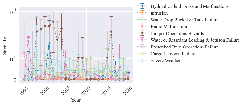
For readability, we define a subset of nine hazards for the graphic analysis.
[28]:
hazards_for_analysis = ['Hydraulic Fluid Leaks and Malfunctions', 'Intrusion', 'Water Drop Bucket or Tank Failure','Radio Malfunction',
                       'Jumper Operations Hazards', 'Water or Retardant Loading & Jettison Failure', 'Prescribed Burn Operations Failure',
                       'Cargo Letdown Failure', 'Severe Weather']
The corresponding frequency, docs, severities, rates, and hazard variables are updated according to the hazards of interest:
[29]:
#update: frequency, docs, severities, rates, hazards
frequency = {hazard: frequency[hazard] for hazard in hazards_for_analysis}
docs = {hazard: docs[hazard] for hazard in hazards_for_analysis}
severities = {hazard: severities[hazard] for hazard in hazards_for_analysis}
rates = {hazard: rates[hazard] for hazard in hazards_for_analysis}
hazards = hazards_for_analysis
To graph the time series, we first define a list of markers and linestyles to use for the hazards:
[30]:
markers = ['.','.','.', 'v', 'v','v', 'x', 'x', 'x']
line_styles = ['--', ':','-.','--', ':','-.','--', ':','-.']
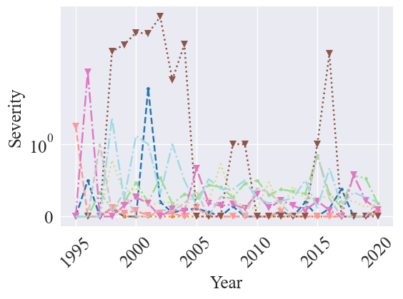
Severity Graphs
Here we graph the severity time series using a logarithmic scale:
[31]:
# legend_kwargs = dict(bbox_to_anchor=(0.5,-0.85), loc="lower center", #mode="expand",# borderaxespad=0,
#                       ncol=3, fontsize=26)
legend_kwargs = {}
plot_metric_time_series(metric_data=severities, metric_name="Severity", fontsize=18, line_styles=line_styles, markers=markers, title="", yscale='log', time_name='Year', show_std=False, save=True, legend=False, legend_kwargs=legend_kwargs, figsize=(6,4))
[32]:
metric_percentage = {hazard: full_metrics.at[hazard, 'F1'] for hazard in hazards_for_analysis}
bootstrap_kwargs={'metric_percentages':metric_percentage, 'num_means':1000, 'CI_interval':95}
plot_metric_time_series(metric_data=severities, metric_name="Severity", line_styles=line_styles, markers=markers, title="", yscale='log', time_name='Year', show_std=False, save=False, bootstrap=True, bootstrap_kwargs=bootstrap_kwargs)
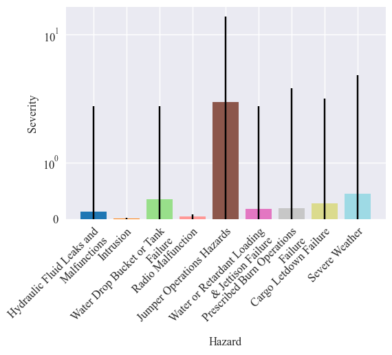
next, we graph the average severity over the years:
[33]:
plot_metric_averages(metric_data=severities, metric_name="Severity", show_std=True, title="", save=False, yscale="log", legend=False, fontsize=12, error_bars='CI')
Frequency Graphs
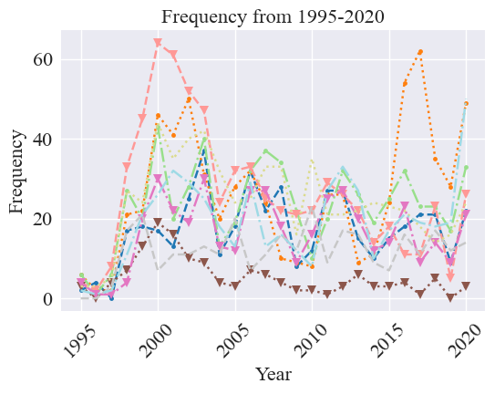
Now we graph the time series of hazard frequency:
[34]:
plot_frequency_time_series(frequency, metric_name='Frequency', line_styles=line_styles, markers=markers, title="Frequency from 1995-2020", time_name="Year", scale=False, save=False, legend=False)
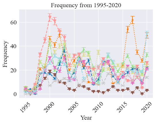
[35]:
false_pos = {hazard: 1-full_metrics.at[hazard, 'Precision'] for hazard in hazards_for_analysis}
false_neg= {hazard: 1-full_metrics.at[hazard, 'Recall'] for hazard in hazards_for_analysis}
#interval_kwargs = {'false_pos_rate':false_pos, 'false_neg_rate':false_neg}
plot_frequency_time_series(frequency, metric_name='Frequency', line_styles=line_styles, markers=markers, title="Frequency from 1995-2020", time_name="Year", scale=False, save=False, legend=False, interval=True)#, interval_kwargs=interval_kwargs)
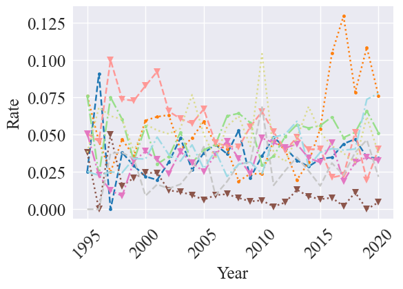
As a comparison, we also graph the rate:
[36]:
plot_frequency_time_series(rates, metric_name='Rate', line_styles=line_styles, fontsize=18, markers=markers, title="", time_name="Year", scale=False, save=True, legend=False, legend_kwargs=legend_kwargs, figsize=(6,4))
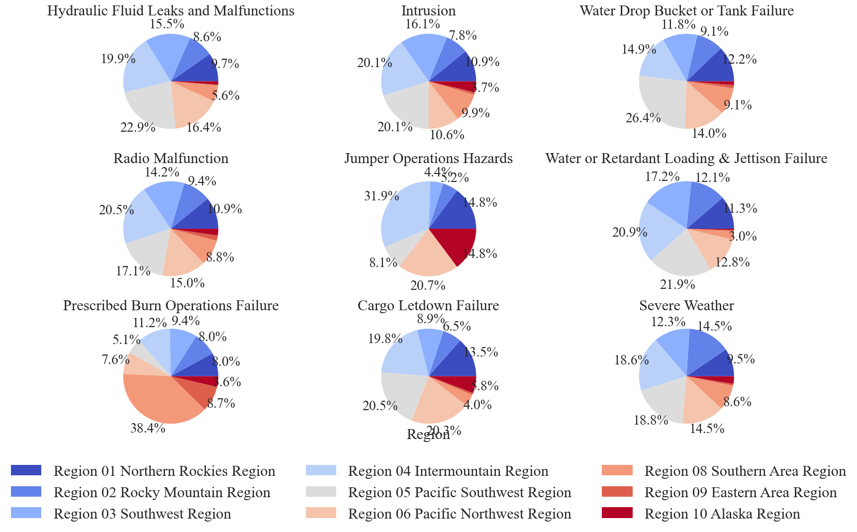
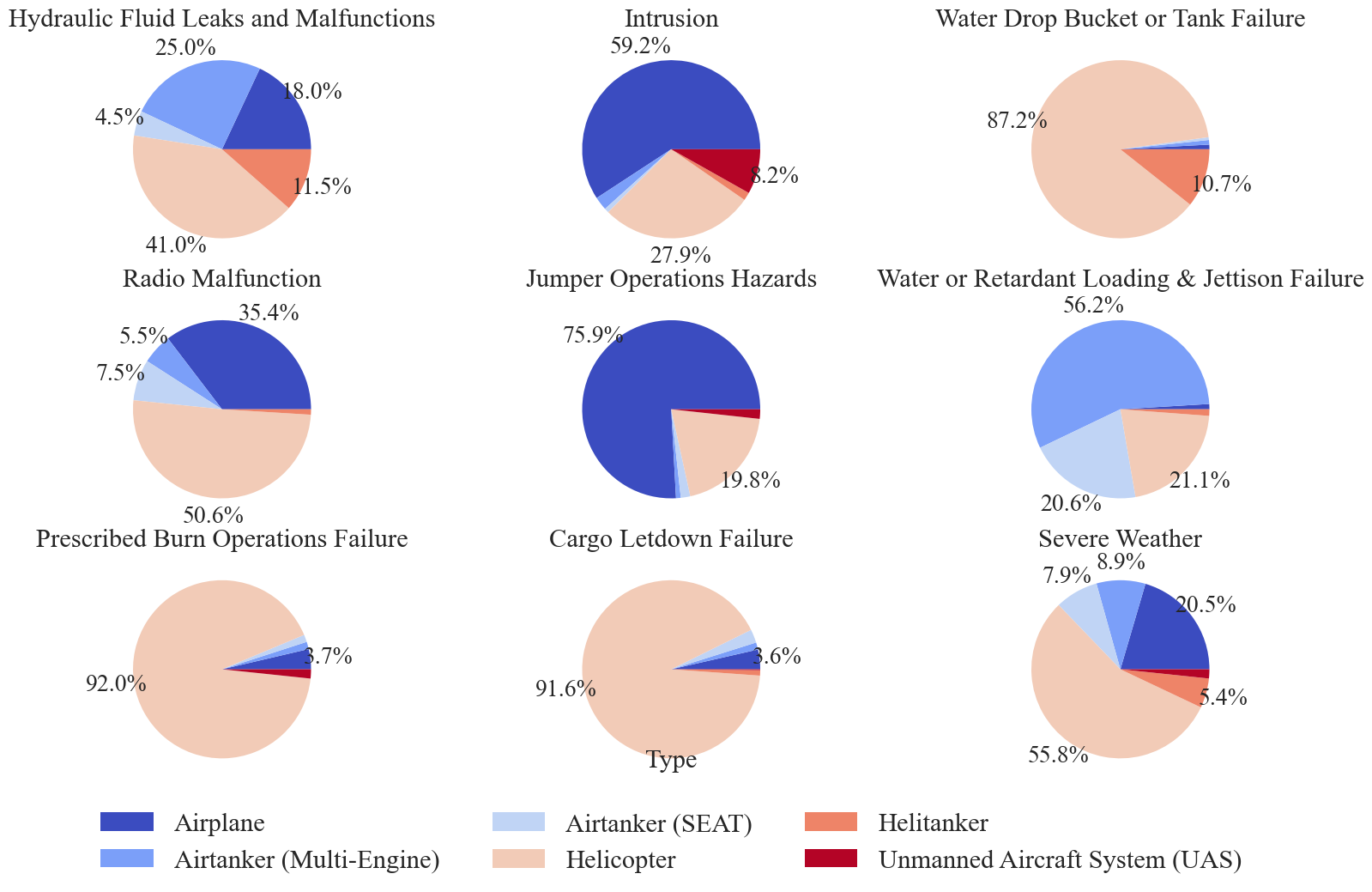
Pie Charts
pie charts are graphed for the region and aircraft type categorical variables. Other variables of interest could include ‘Manufacturer’, ‘Model’, and ‘Mission Type’.
[37]:
predictors = ['region_corrected', 'Type']
pie_kwargs = {'pctdistance':1.2}

for predictor in predictors:
    if predictor == 'region_corrected':
        predictor_label='Region'
        padding = 1
        legend_kwargs = dict(bbox_to_anchor=(0.5,-0.2), loc="lower center", ncol=3)
    else:
        predictor_label = None
        padding = 0
        legend_kwargs = dict(bbox_to_anchor=(0.5,-0.15), loc="lower center", ncol=3)
    make_pie_chart(docs, preprocessed_df, predictor, hazards, 'Tracking #', predictor_label, save=True, fontsize=22, padding=padding, pie_kwargs=pie_kwargs, legend_kwargs=legend_kwargs)
Secondary Analysis
The secondary analysis is performed to determine if trends in the graphic analysis are statistically significant. Additionally a risk matrix is produced in this part of the analysis. This step includes: - chi-squared analysis - ANOVA - Risk matrix
Chi-Squared Analysis
The chi-squared analysis determines if the distribution of a categorical variable, such as region, is dependent on another variable, such as the presence of a hazard. Essentially this test can determine if a hazard occurs more or less often in a certain categorical variable condition (e.g., a specific region) when compared to the complete dataset. Here we run the chi-squared test for region and aircraft type over each hazard.
To do this, we must first add hazard occurrence to the preprocessed dataframe:
[38]:
#add hazard values to preprocessed_df
preprocessed_df = add_hazards_to_docs(preprocessed_df, "Tracking #", docs)
Now we run the chi-squared tests, which out put a statistics dataframe and a counts dataframe
[39]:
pred_dict = {'region_corrected':'Region', 'Type': "Aircraft Type", 'Agency':'Agency'}
stats_df, count_dfs = chi_squared_tests(preprocessed_df, hazards, predictors, pred_dict)
The resulting stats_df contains the chi-squared statistic an p-value for each hazard and predictor. A significant p-value indicates the distribution of the predictor across reports with the hazard is different than the distribution of the predictor accross reports without the hazard.
[40]:
stats_df
[40]:
| Predictor | Region | Aircraft Type | ||
|---|---|---|---|---|
| Measure | p-val | chi-squared | p-val | chi-squared |
| Hydraulic Fluid Leaks and Malfunctions | 0.001 | 28.908 | 0.0 | 134.778 |
| Intrusion | 0.004 | 24.521 | 0.0 | 1136.508 |
| Water Drop Bucket or Tank Failure | 0.002 | 26.431 | 0.0 | 462.073 |
| Radio Malfunction | 0.018 | 19.994 | 0.0 | 194.557 |
| Jumper Operations Hazards | 0.000 | 116.608 | 0.0 | 249.196 |
| Water or Retardant Loading & Jettison Failure | 0.000 | 50.256 | 0.0 | 936.333 |
| Prescribed Burn Operations Failure | 0.000 | 467.884 | 0.0 | 194.023 |
| Cargo Letdown Failure | 0.000 | 53.263 | 0.0 | 391.816 |
| Severe Weather | 0.009 | 22.069 | 0.0 | 27.198 |
To futher examine these differences, we display the counts df. Negative count values indicate the condition occurs less there than expected, whereas positive values have the condition occur more. For example, there are more reports with hydraulic fluid leaks in region 5 than expected.
[41]:
for df in count_dfs:
    display(count_dfs[df])
| Region 05 Pacific Southwest Region | Region 04 Intermountain Region | Region 06 Pacific Northwest Region | Region 03 Southwest Region | Region 01 Northern Rockies Region | Region 02 Rocky Mountain Region | Region 08 Southern Area Region | Region 10 Alaska Region | Region 09 Eastern Area Region | |||
|---|---|---|---|---|---|---|---|---|---|---|---|
| Hazard | Present | ||||||||||
| Hydraulic Fluid Leaks and Malfunctions | 0 | -10.638116 | -12.806310 | -5.569277 | -12.981197 | 1.322365 | -0.045415 | 11.523624 | 15.625926 | 9.416939 | 4.151462 |
| 1 | 10.638116 | 12.806310 | 5.569277 | 12.981197 | -1.322365 | 0.045415 | -11.523624 | -15.625926 | -9.416939 | -4.151462 | |
| Intrusion | 0 | 9.034818 | -13.801928 | 33.510398 | -17.671022 | -1.775237 | 7.637638 | -7.516772 | -10.879452 | -1.294319 | 2.755876 |
| 1 | -9.034818 | 13.801928 | -33.510398 | 17.671022 | 1.775237 | -7.637638 | 7.516772 | 10.879452 | 1.294319 | -2.755876 | |
| Water Drop Bucket or Tank Failure | 0 | -25.347383 | 17.113059 | 11.601068 | 8.147956 | -8.336308 | 0.040953 | -1.896741 | -14.820572 | 12.522269 | 0.975699 |
| 1 | 25.347383 | -17.113059 | -11.601068 | -8.147956 | 8.336308 | -0.040953 | 1.896741 | 14.820572 | -12.522269 | -0.975699 | |
| Radio Malfunction | 0 | 28.822006 | -15.149869 | 7.093299 | -5.189786 | -1.389292 | -2.033145 | -0.200303 | -16.588798 | 7.834117 | -3.198231 |
| 1 | -28.822006 | 15.149869 | -7.093299 | 5.189786 | 1.389292 | 2.033145 | 0.200303 | 16.588798 | -7.834117 | 3.198231 | |
| Jumper Operations Hazards | 0 | 16.157995 | -20.503944 | -7.889889 | 10.602661 | -6.684886 | 4.357979 | 10.918174 | 7.027568 | -15.568959 | 1.583300 |
| 1 | -16.157995 | 20.503944 | 7.889889 | -10.602661 | 6.684886 | -4.357979 | -10.918174 | -7.027568 | 15.568959 | -1.583300 | |
| Water or Retardant Loading & Jettison Failure | 0 | -4.967652 | -15.392638 | 10.224763 | -18.627998 | -4.800335 | -13.856107 | 21.783045 | 10.027328 | 11.710541 | 3.899052 |
| 1 | 4.967652 | 15.392638 | -10.224763 | 18.627998 | 4.800335 | 13.856107 | -21.783045 | -10.027328 | -11.710541 | -3.899052 | |
| Prescribed Burn Operations Failure | 0 | 47.203888 | 19.697634 | 24.320612 | 11.416142 | 8.007250 | 3.596606 | -81.394550 | -12.401641 | -0.014102 | -20.431838 |
| 1 | -47.203888 | -19.697634 | -24.320612 | -11.416142 | -8.007250 | -3.596606 | 81.394550 | 12.401641 | 0.014102 | 20.431838 | |
| Cargo Letdown Failure | 0 | 6.194965 | -10.952673 | -24.775874 | 24.313521 | -16.599554 | 14.522428 | 26.527368 | -9.512628 | -12.899769 | 3.182217 |
| 1 | -6.194965 | 10.952673 | 24.775874 | -24.313521 | 16.599554 | -14.522428 | -26.527368 | 9.512628 | 12.899769 | -3.182217 | |
| Severe Weather | 0 | 11.201737 | -4.655565 | 5.716995 | 3.034260 | 4.146682 | -25.930205 | -0.520516 | 0.259103 | 4.022389 | 2.725122 |
| 1 | -11.201737 | 4.655565 | -5.716995 | -3.034260 | -4.146682 | 25.930205 | 0.520516 | -0.259103 | -4.022389 | -2.725122 |
| Helicopter | Airplane | Airtanker (Multi-Engine) | Airtanker (SEAT) | Helitanker | Unmanned Aircraft System (UAS) | |||
|---|---|---|---|---|---|---|---|---|
| Hazard | Present | |||||||
| Hydraulic Fluid Leaks and Malfunctions | 0 | 51.354075 | 15.874432 | -48.860489 | 3.288901 | -34.007330 | 9.416939 | 2.933471 |
| 1 | -51.354075 | -15.874432 | 48.860489 | -3.288901 | 34.007330 | -9.416939 | -2.933471 | |
| Intrusion | 0 | 180.330412 | -218.654530 | 78.555255 | 30.063023 | 16.583619 | -41.294319 | -45.583459 |
| 1 | -180.330412 | 218.654530 | -78.555255 | -30.063023 | -16.583619 | 41.294319 | 45.583459 | |
| Water Drop Bucket or Tank Failure | 0 | -207.010517 | 124.825512 | 79.144371 | 28.535973 | -40.989881 | 11.522269 | 3.972273 |
| 1 | 207.010517 | -124.825512 | -79.144371 | -28.535973 | 40.989881 | -11.522269 | -3.972273 | |
| Radio Malfunction | 0 | 41.409290 | -72.800414 | 60.108836 | -10.729504 | 19.735001 | -42.165883 | 4.442674 |
| 1 | -41.409290 | 72.800414 | -60.108836 | 10.729504 | -19.735001 | 42.165883 | -4.442674 | |
| Jumper Operations Hazards | 0 | 48.721297 | -58.533025 | 18.098558 | 5.157836 | 5.222691 | -17.568959 | -1.098399 |
| 1 | -48.721297 | 58.533025 | -18.098558 | -5.157836 | -5.222691 | 17.568959 | 1.098399 | |
| Water or Retardant Loading & Jettison Failure | 0 | 132.920245 | 87.176799 | -177.905187 | -64.852203 | 11.160067 | 8.710541 | 2.789738 |
| 1 | -132.920245 | -87.176799 | 177.905187 | 64.852203 | -11.160067 | -8.710541 | -2.789738 | |
| Prescribed Burn Operations Failure | 0 | -115.367222 | 55.407458 | 39.040953 | 12.131065 | 11.769978 | -0.014102 | -2.968130 |
| 1 | 115.367222 | -55.407458 | -39.040953 | -12.131065 | -11.769978 | 0.014102 | 2.968130 | |
| Cargo Letdown Failure | 0 | -239.655565 | 111.669030 | 78.635487 | 17.469604 | 17.691339 | 11.100231 | 3.089873 |
| 1 | 239.655565 | -111.669030 | -78.635487 | -17.469604 | -17.691339 | -11.100231 | -3.089873 | |
| Severe Weather | 0 | -10.659947 | 7.550872 | 26.059278 | -12.117680 | -7.115051 | 1.022389 | -4.739861 |
| 1 | 10.659947 | -7.550872 | -26.059278 | 12.117680 | 7.115051 | -1.022389 | 4.739861 |
ANOVA
An ANOVA is performed to determine if there is a statistically siginificant difference in severity between the hazards.
To perform this, we first format the data into an AOV_df, which allows us to easily run the test.
[42]:
severities_dict = {hazard:[] for hazard in hazards}
AOV_df = {'hazard':[], 'severity':[]}
for hazard in hazards:
    hazard_df = preprocessed_df.loc[preprocessed_df[hazard] == 1]
    sevs = hazard_df['severity'].tolist()
    severities_dict[hazard] = sevs
    for sev in sevs:
        AOV_df['hazard'].append(hazard)
        AOV_df['severity'].append(sev)
AOV_df = pd.DataFrame(AOV_df)
Now that the data is formatted, we run the test. The Welch ANOVA is chosen because the data does not meet the criteria for a conventional ANOVA (same variances/sample sizes). The first ANOVA test we run checks if the severity between hazard and non-hazard documents is different for each hazard and the anova result is displayed.
[43]:
anovas = []
for hazard in hazards:
    aov = pg.welch_anova(dv='severity', between=hazard, data=preprocessed_df).round(3)
    anovas.append(aov)
anova_results = pd.concat(anovas)
anova_results
[43]:
| Source | ddof1 | ddof2 | F | p-unc | np2 | |
|---|---|---|---|---|---|---|
| 0 | Hydraulic Fluid Leaks and Malfunctions | 1 | 478.828 | 2.661 | 0.103 | 0.000 |
| 0 | Intrusion | 1 | 5701.889 | 358.199 | 0.000 | 0.002 |
| 0 | Water Drop Bucket or Tank Failure | 1 | 699.347 | 17.853 | 0.000 | 0.001 |
| 0 | Radio Malfunction | 1 | 1487.105 | 120.882 | 0.000 | 0.002 |
| 0 | Jumper Operations Hazards | 1 | 137.102 | 26.684 | 0.000 | 0.045 |
| 0 | Water or Retardant Loading & Jettison Failure | 1 | 503.159 | 0.870 | 0.351 | 0.000 |
| 0 | Prescribed Burn Operations Failure | 1 | 336.694 | 0.272 | 0.602 | 0.000 |
| 0 | Cargo Letdown Failure | 1 | 739.366 | 5.336 | 0.021 | 0.000 |
| 0 | Severe Weather | 1 | 512.122 | 11.595 | 0.001 | 0.002 |
Next we run an anova between all of the hazards, resulting in one F value. This test determines if there is a difference in severity between any of the hazards.
[44]:
aov = pg.welch_anova(dv='severity', between='hazard', data=AOV_df).round(3)
[45]:
aov
[45]:
| Source | ddof1 | ddof2 | F | p-unc | np2 | |
|---|---|---|---|---|---|---|
| 0 | hazard | 8 | 1266.871 | 33.264 | 0.0 | 0.096 |
Since the ANOVA yeiled a significant result, we want to further determine which hazards are more severe than others. We do this using pairwise testing, in this case the gameshowell test.
[46]:
post_hoc = pg.pairwise_gameshowell(dv='severity', between='hazard', data=AOV_df).round(3)
To simplify the results output, we filter out the results to only show hazard pairs that have a significant difference in severity
[47]:
post_hoc = post_hoc.loc[post_hoc['pval']<0.05].reset_index(drop=True)
[48]:
post_hoc = post_hoc[['A', 'B', 'df', 'T', 'pval', 'hedges']]
post_hoc.index = post_hoc['A']
post_hoc = post_hoc.drop(['A'], axis=1)
post_hoc
[48]:
| B | df | T | pval | hedges | |
|---|---|---|---|---|---|
| A | |||||
| Cargo Letdown Failure | Intrusion | 674.026 | 8.586 | 0.000 | 0.493 |
| Cargo Letdown Failure | Jumper Operations Hazards | 138.706 | -4.914 | 0.000 | -0.931 |
| Cargo Letdown Failure | Radio Malfunction | 850.972 | 7.120 | 0.000 | 0.405 |
| Hydraulic Fluid Leaks and Malfunctions | Jumper Operations Hazards | 141.275 | -5.268 | 0.000 | -0.864 |
| Hydraulic Fluid Leaks and Malfunctions | Severe Weather | 852.553 | -3.627 | 0.009 | -0.230 |
| Hydraulic Fluid Leaks and Malfunctions | Water Drop Bucket or Tank Failure | 835.475 | -3.681 | 0.008 | -0.236 |
| Intrusion | Jumper Operations Hazards | 137.067 | -5.619 | 0.000 | -1.160 |
| Intrusion | Prescribed Burn Operations Failure | 322.167 | -4.002 | 0.003 | -0.390 |
| Intrusion | Severe Weather | 504.976 | -6.002 | 0.000 | -0.411 |
| Intrusion | Water Drop Bucket or Tank Failure | 647.167 | -9.938 | 0.000 | -0.583 |
| Intrusion | Water or Retardant Loading & Jettison Failure | 459.811 | -5.436 | 0.000 | -0.411 |
| Jumper Operations Hazards | Prescribed Burn Operations Failure | 140.431 | 5.136 | 0.000 | 0.769 |
| Jumper Operations Hazards | Radio Malfunction | 137.315 | 5.537 | 0.000 | 1.134 |
| Jumper Operations Hazards | Severe Weather | 146.659 | 4.419 | 0.001 | 0.682 |
| Jumper Operations Hazards | Water Drop Bucket or Tank Failure | 139.025 | 4.735 | 0.000 | 0.881 |
| Jumper Operations Hazards | Water or Retardant Loading & Jettison Failure | 138.697 | 5.168 | 0.000 | 0.868 |
| Prescribed Burn Operations Failure | Radio Malfunction | 368.341 | 3.190 | 0.041 | 0.281 |
| Radio Malfunction | Severe Weather | 531.014 | -5.509 | 0.000 | -0.374 |
| Radio Malfunction | Water Drop Bucket or Tank Failure | 793.955 | -8.538 | 0.000 | -0.495 |
| Radio Malfunction | Water or Retardant Loading & Jettison Failure | 586.598 | -4.166 | 0.001 | -0.291 |
| Severe Weather | Water or Retardant Loading & Jettison Failure | 665.899 | 3.399 | 0.020 | 0.211 |
| Water Drop Bucket or Tank Failure | Water or Retardant Loading & Jettison Failure | 1024.937 | 3.707 | 0.007 | 0.224 |
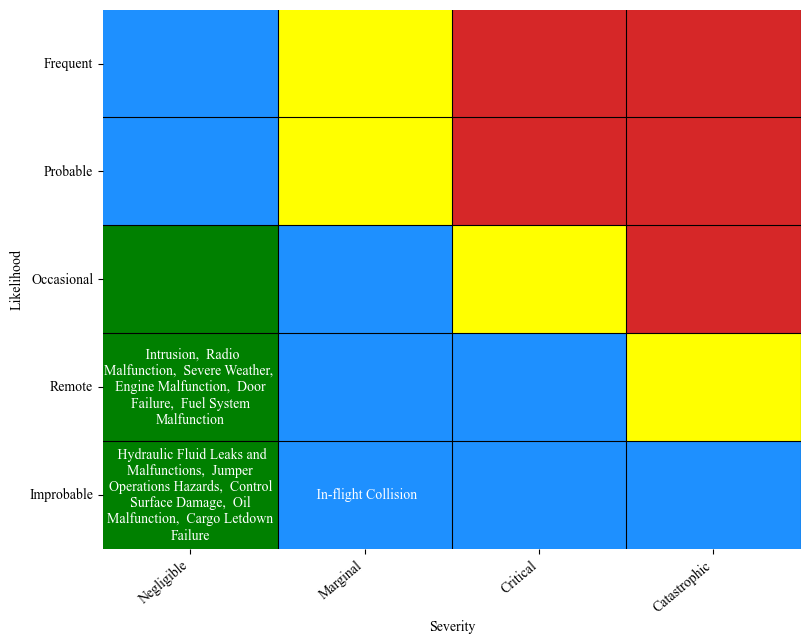
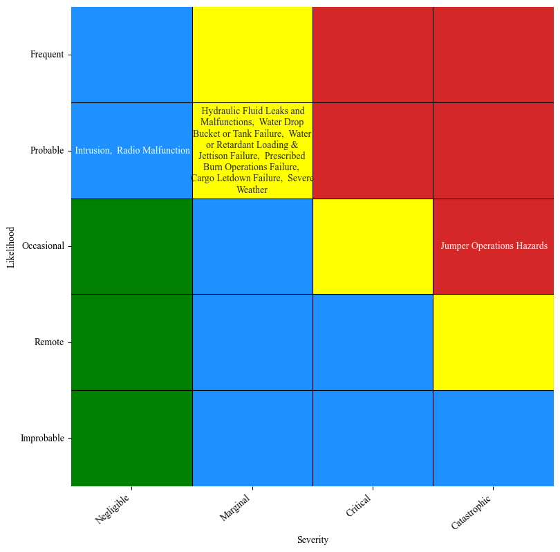
Risk Matrix
To display this infomation in an accessible format, we place the hazards on a risk matrix according to USFS guidelines.
First, configure the plotting parameters:
[49]:
import matplotlib as mpl
mpl.rcParams.update(mpl.rcParamsDefault)
plt.rcParams["font.family"] = "Times New Roman"
Next, assign likelihood and severity categories using the numeric hazard severity and rate values previously calculated:
[50]:
severities = table['Severity']
severities.index = table['Hazards']
severities_raw = severities[hazards]
severities_raw = severities_raw.to_dict()
#severities = get_SAFECOM_severity_FAA(severities_raw)
rates = table['Rate']
rates.index = table['Hazards']
rates = rates[hazards]
rates = rates.to_dict()
#likelihood = get_likelihood_FAA(rates)
[51]:
severities_USFS = get_SAFECOM_severity_USFS(severities_raw)
likelihood = get_likelihood_USFS(rates)
Now we can plot the risk matrix using the defined categories:
[52]:
plot_USFS_risk_matrix(likelihood, severities_USFS, figsize=(9,9), save=False, results_path="SAFECOM_JAIS_USFS_risk_matrix", fontsize=10, max_chars=30, title=False)
Situation Specific Risk Matrices
To demonstrate the usefulness of this framework, we present a case study of situation specific risk matrices developed from SAFECOM reports.
Here we define the functions needed to create these risk matrices. They include filtering the dataframe based on a set of conditions, then recalculating the hazard rate and severity for each hazard.
[53]:
def filter_df(df, filters):
    for col in filters:
        df = df.dropna(subset=[col])
        df = df[df[col].apply(lambda x: filters[col] in x)].reset_index(drop=True)
    return df
[54]:
def get_custom_rm(df, filters, hazard_file, results_file, keep_hazards=[], save=False):
    preprocessed_df = filter_df(df, filters)
    frequency, docs, hazard_words_per_doc, topics_per_doc, hazard_topics_per_doc = identify_docs_per_hazard(hazard_file, preprocessed_df, results_file, 'Narrative', 'Year', "Tracking #", 'Narrative', doc_topic_dist_field='document topic distribution', topic_thresh=0.2)
    rates = calc_rate(frequency)
    _, severities = calc_severity_per_hazard(docs, preprocessed_df, id_field='Tracking #')
    #replace nans with 0
    severities = {hazard:severities[hazard] if (not np.isnan(severities[hazard])) else 0 for hazard in severities}
    if keep_hazards == []:
        keep_hazards = [hazard for hazard in docs]
    #rm extra hazards
    severities = {hazard: severities[hazard] for hazard in severities if hazard in keep_hazards}
    rates = {hazard: rates[hazard] for hazard in rates if hazard in keep_hazards}
    severities_USFS = get_SAFECOM_severity_USFS(severities)
    likelihood = get_likelihood_USFS(rates)
    filters_string = ""
    for key in filters:
        filters_string += key.replace(" ", "_")
        filters_string += filters[key].replace(" ", "_")
    results_path = 'risk_matrix_'+filters_string+'.pdf'
    plot_USFS_risk_matrix(likelihood, severities_USFS, figsize=(9,7), save=save, results_path=results_path, fontsize=10, max_chars=28, title=False)
Example 1: Aerial commander flying an Aero Commander airplane in California
We define the hazards to include on the custom risk matrix:
[55]:
keep_hazards = ['Hydraulic Fluid Leaks and Malfunctions','Intrusion','Airspace Control Hazards','Radio Malfunction','Jumper Operations Hazards',
                'Cargo Letdown Failure','Severe Weather',
               'Fuel System Malfunction', 'Landing Gear Malfunction', 'Engine Malfunction', 'Oil Malfunction', 'Control Surface Damage',
               'In-flight Collision', 'Door Failure']
Next we specify the featues that define the scenario and get the custom risk matrix:
[56]:
filters ={"Mission Type":'Fire, Air Attack',
          "Type":'Airplane',
         "Manufacturer":'Aero Commander',
         "region_corrected":'Region 05 Pacific Southwest Region'}
get_custom_rm(preprocessed_df, filters, hazard_file, results_file, keep_hazards)
100%|██████████| 26/26 [00:02<00:00, 9.31it/s]

Example 2: Air Tanker flying a redardant drop mission with a Lockheed multi-engine in Oregon
Again, specify the filters that define the scenario then get the risk matrix:
[57]:
filters ={"Mission Type":'Fire, Retardant Drop (Airtanker)',
         "Type":'Airtanker (Multi-Engine)',
          "Manufacturer": "Lockheed",
         'region_corrected':'Region 06 Pacific Northwest Region'}
keep_hazards = ['Hydraulic Fluid Leaks and Malfunctions','Intrusion','Water Drop Bucket or Tank Failure','Radio Malfunction','Jumper Operations Hazards',
                'Water or Retardant Loading & Jettison Failure', 'Cargo Letdown Failure','Severe Weather',
               'Fuel System Malfunction', 'Landing Gear Malfunction', 'Engine Malfunction', 'Oil Malfunction', 'Control Surface Damage',
               'In-flight Collision', 'Door Failure']
get_custom_rm(preprocessed_df, filters, hazard_file, results_file, keep_hazards)
100%|██████████| 26/26 [00:01<00:00, 17.33it/s]

Example 3: Pilot flying a Bell Helicopter for reconnaisance in Texas
In addition to specifying the filters, for this risk matrix we also define a new list of hazards that are more relevant to this scenario:
[58]:
filters ={"Mission Type":'Fire, Reconnaissance',
         "Type":'Helicopter',
          "Manufacturer": "Bell",
          #"Model":"600",#includes 600
          'region_corrected':'Region 08 Southern Area Region'}
keep_hazards = ['Hydraulic Fluid Leaks and Malfunctions','Intrusion', 'Radio Malfunction','Jumper Operations Hazards',
                'Cargo Letdown Failure','Severe Weather',
               'Fuel System Malfunction', 'Engine Malfunction', 'Oil Malfunction', 'Control Surface Damage',
               'In-flight Collision', 'Door Failure']
get_custom_rm(preprocessed_df, filters, hazard_file, results_file, keep_hazards)
100%|██████████| 26/26 [00:01<00:00, 21.08it/s]