This will copy all of the files into a newly created work/ folder. Follow
the instructions below by entering that work/ folder; the purpose is that
you can easily delete the work/ folder and restart the tutorial at any
time.
To keep computation time low for the purposes of running examples. The example
seeks to introduce the pyFun user to data books and automated reports,
including sweep plots. It should be noted that the Cart3D examples are more descriptive, and users are encouraged to consider
reading those examples since most of the process is the same for each solver.
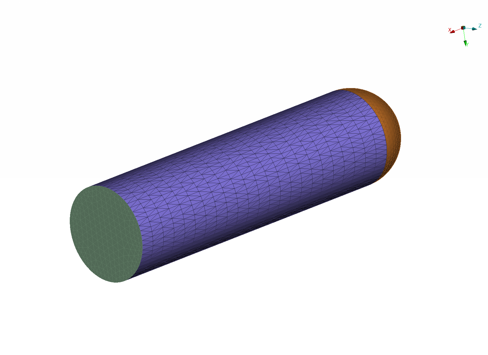
The geometry used for this shape is a capped cylinder and little or nothing
else. An inviscid volume mesh was created using AFLR3. The surface
triangulation, bullet.tri, is shown below.
Figure 5.2 Simple bullet shape triangulation with four fins
The files in this folder are listed below with a short description. In this
case, the run matrix is defined within the pyFun.json file.
pyFun.json: Master input control file for pyFun
matrix.csv: Run matrix
fun3d.nml: Template namelist file
bullet-inviscid.ugrid: Volume grid, ASCII AFLR3 format
Assuming the present working directory is in this demo folder, i.e.
pyfun02_bullet, a good first test command is the following, which checks
the status of each case in the matrix.
$ pyfun-c
Case Config/Run Directory Status Iterations Que CPU Time---- --------------------- ------- ----------- --- --------0 bullet/m0.80a0.0b0.0 --- / .1 bullet/m0.80a4.0b0.0 --- / ....23 bullet/m1.75a30.0b0.0 --- / .---=24,
This example contains 24 cases in the run matrix, and the computation time is
kept low in order to run each case within a few minutes (using the serial
version of FUN3D).
Running case number 3 (note zero-based indexing) has the following output.
$ pyfun-I3Case Config/Run Directory Status Iterations Que CPU Time---- --------------------- ------- ----------- --- --------3 bullet/m0.80a30.0b0.0 --- / . Case name: 'bullet/m0.80a30.0b0.0' (index 3) Starting case 'bullet/m0.80a30.0b0.0' > nodet --animation_freq 100 (PWD = 'bullet/m0.80a30.0b0.0') (STDOUT = 'fun3d.out') > nodet --animation_freq 100 (PWD = 'bullet/m0.80a30.0b0.0') (STDOUT = 'fun3d.out')Submitted or ran 1 job(s).---=1,
We can then check how much CPU time that used.
$ pyfun-I3-c
Case Config/Run Directory Status Iterations Que CPU Time---- --------------------- ------- ----------- --- --------3 bullet/m0.80a30.0b0.0 DONE 200/200 . 0.1DONE=1,
In the master input file pyFun.json, the key section is the "Fun3D"
section, which modifies the template namelist fun3d.nml. The example
is set up to run two phases. The first phase has a starting CFL number of 0.1
which ramps up to 100.0. The second phase has a constant CFL number of 100.0.
Another interesting parameter is the Config>File, which is set to
"bullet.xml". This is an XML file that prescribes a name for each
component and furthermore can be used to define groups of components. While
this is not a recognized FUN3D file format, it is used by pyFun to make some of
the setup easier. Some of the text from the XML file are shown below.
In particular, this allows pyFun to set the correct namelist parameters to
track the forces and moments on each component. This is important because
FUN3D internally renumbers all the components 1,2,…,*N* according to the
lines of the .mapbc file. The present setup in the Config section of
pyFun.json prevents the need to figure out the component number(s) for
each component.
Before moving on to the next session, let’s also run case 17 so we can complete
the rest of the tutorial. Some of the aerodynamic data book is already in
place, but cases 3 and 17 are missing. Users may wish to run all 24 cases or
just a few more in order to do more experimenting.
This example is set up to create a report called report-case.pdf in the
report/ folder. It includes a couple of summary tables, 8 iterative
history plots, and a flow visualization slide that works with Paraview.
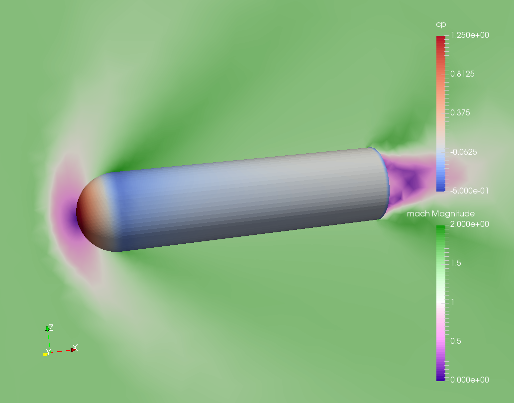
Figure 5.3 shows an example of this Paraview image from
case 17 (bullet/m1.50a4.0b0.0).
Figure 5.3 Surface \(c_p\) and \(y{=}0\) Mach slice
Note about Paraview figure: This example requires
ParaView with VisIt Bridge
since it reads binary Tecplot (.plt) files. Installation can be tricky,
and prepackaged ParaView modules often do not have the VisIt bridge. One
relatively easy workaround is to install the free and open-source software
SALOME, which
does include the appropriate version. It is fairly simple to download a
version of SALOME and then use the included ParaView binaries within that
installation.
The report also includes axial force coefficient (CA), side force coefficient
(CY), and normal force (CY) coefficient on both bullet_no_base and
cap. The bullet_no_base component includes bot the rounded nose
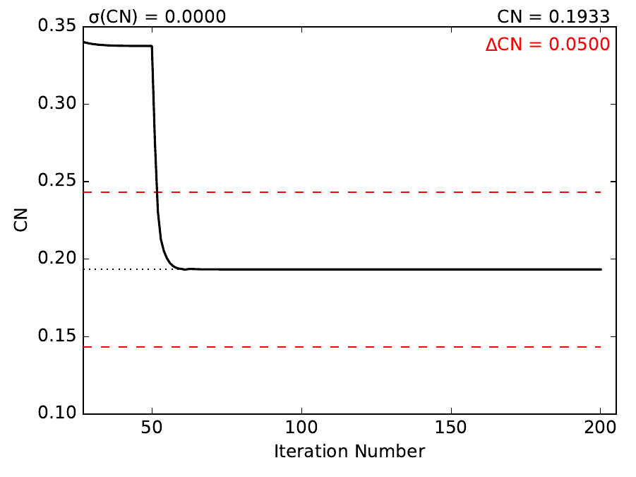
cap and the cylindrical portion. Figure 5.4 shows
one of these plots.
Figure 5.4 Iterative history on bullet (not including base) normal force
coefficient (CN) for bullet/m1.50a4.0b0.0
In addition, there is a plot of overall pitching moment coefficient, and a
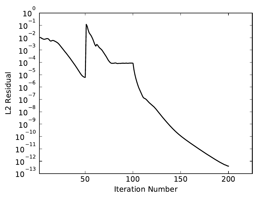
residual plot. Both Figure 5.4 and
Figure 5.5 show a big change of behavior at iteration 50, when
the first-order iterations end. The residual history also shows a change of
behavior at iteration 75; the residual stops dropping for a while while the
fluxes are frozen.
Figure 5.5 Overall \(L_2\) residual for bullet/m1.50a4.0b0.0
The Paraview subfigure settings from the JSON file are shown below.
"slice-y0":{"Type":"Paraview","Caption":"Surface $c_p$ and $y{=}0$ Mach slice","Width":0.33,"Layout":"slice-y0.py","ImageFile":"slice-y0.png"}
This points pyFun to the Python script slice-y0.py. The image is
created by the system command pvpythonslice-y0.py in each case folder.
This slice-y0.py was created by recording a Python script in
ParaView interactively and then modifying the resulting script later. At the
time of writing, this is found in the Tools menu under Tools>Start Trace.
The header of this script contains some helper functions that were added in
order to provide a solution for users who do not have a version of FUN3D
compiled with the TecIO library. It does require the user to use Tecplot’s
preplot tool, which can be downloaded from the Tecplot TecIO library
website. The first few
lines of slice-y0.py are shown below.
#### import the simple module from the paraviewfromparaview.simpleimport*#### disable automatic camera reset on 'Show'paraview.simple._DisableFirstRenderCameraReset()# System interfaceimportos# Check for DAT instead of PLT fileforfin['arrow_tec_boundary','arrow_plane-y0']:# Name of DAT and PLT filesfdat='%s.dat'%ffplt='%s.plt'%f# Check for DAT fileifos.path.isfile(fdat):# Delete any PLT fileifos.path.isfile(fplt):os.remove(fplt)# Create new PLT fileos.system('preplot %s%s'%(fdat,fplt))
Most of the rest of the contents of the Python script come from the ParaView
API, but the
command at the end is relevant.
# save screenshotSaveScreenshot('slice-y0.png',magnification=1,quality=100,view=renderView1)
This is the command that actually saves the image, and it is relevant to
explain here that the name of the image, 'slice-y0.png', must line up with
the ImageFile option from the JSON subfigure definition.
The provided example in $PYCART/examples/pyfun/02_bullet/ includes an
aerodynamic database for all but two of the 24 conditions in the
data/bullet folder. The contents of an aero data book file are the same
here as for Cart3D, and a selection of text from the main bullet_no_base
file can be seen below. These aero data book files have the file name
aero_$COMP.csv for an arbitrary component COMP.
# Database statistics for 'bullet_no_base' extracted on 2017-04-09 19:35:55
#
#mach,alpha,beta,q,T,config,Label,CA,CY,CN,...,nOrders,nIter,nStats
0.8,0,0,1250,475.33,bullet,,0.1293,-0.0036,-0.0001,...,6.7889,200,50
0.8,4,0,1250,475.33,bullet,,0.1260,-0.0046,0.1854,...,6.8890,200,50
...
1.75,30,0,1250,475.33,bullet,,0.6291,-0.0010,2.8408,...,4.5099,200,50
This is a relatively simple data book definition, as shown in the DataBook
section of pyFun.json, reproduced below. We include five data book
components here, and all are restricted to be just forces to make some of the
files smaller. Normally, a user would not include the lines such as "cap":{"Type":"Force"}. Without a user-specified type, components have the type
"FM", which stand for “Force & Moment” (except for Cart3D data books, which
are by default "Force"). The DataBook>nStats component means that at
least 50 iterations must be included in the averaging window for each
coefficient of each component, and nMin states that only iterations after
iteration 150 are allowed to be included.
"DataBook":{// List of components"Components":["bullet_no_base","bullet_total","cap","body","base"],// Location"Folder":"data/bullet",// Overall statistic inputs"nStats":50,"nMin":150,// Definitions"bullet_no_base":{"Type":"Force"},"bullet_total":{"Type":"Force"},"cap":{"Type":"Force"},"body":{"Type":"Force"},"base":{"Type":"Force"}}
Running the command pyfun--aero will fill in the other two cases.
$ pyfun-I:3--aero
bullet/m0.80a0.0b0.0bullet/m0.80a4.0b0.0bullet/m0.80a10.0b0.0bullet/m0.80a30.0b0.0 Adding new databook entry at iteration 200.bullet/m0.95a0.0b0.0bullet/m0.95a4.0b0.0bullet/m0.95a10.0b0.0bullet/m0.95a30.0b0.0bullet/m1.10a0.0b0.0bullet/m1.10a4.0b0.0bullet/m1.10a10.0b0.0bullet/m1.10a30.0b0.0bullet/m1.25a0.0b0.0bullet/m1.25a4.0b0.0bullet/m1.25a10.0b0.0bullet/m1.25a30.0b0.0bullet/m1.50a0.0b0.0bullet/m1.50a4.0b0.0 Adding new databook entry at iteration 200.bullet/m1.50a10.0b0.0bullet/m1.50a30.0b0.0bullet/m1.75a0.0b0.0bullet/m1.75a4.0b0.0bullet/m1.75a10.0b0.0bullet/m1.75a30.0b0.0
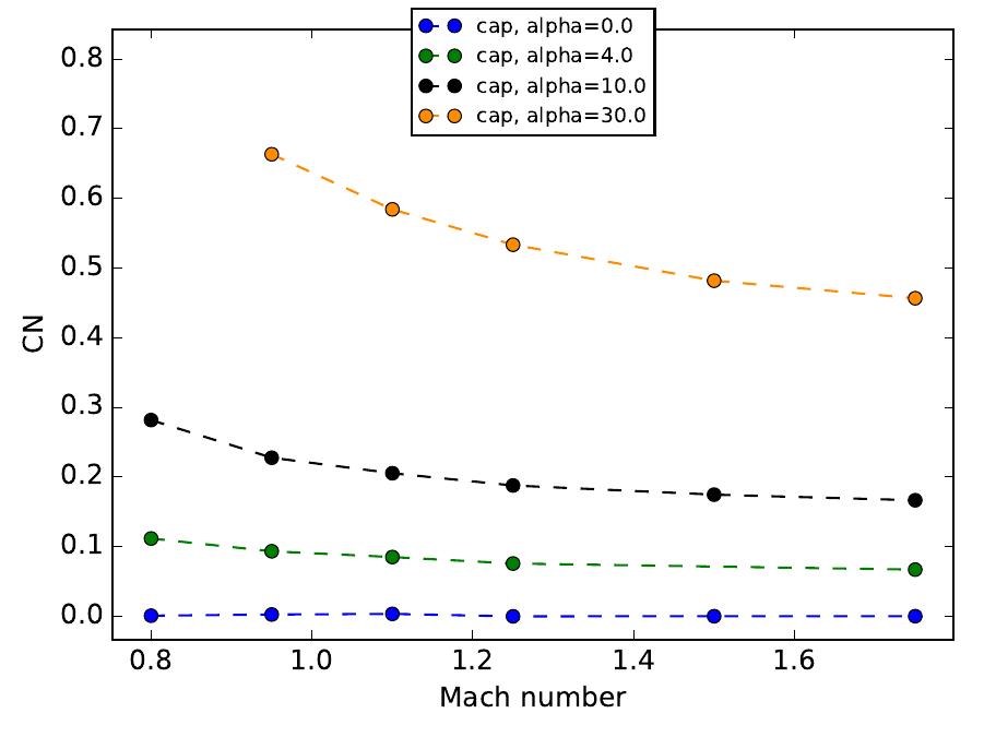
The pyFun.json"Report" section also includes a Mach sweep figure.
Details of the Mach sweep (with an angle of attack carpet plot) are the same as
in the Cart3D example Demo 7: Data Book Plots and Reports, but
Figure 5.6 gives an example of one of the plots from
the resulting report-mach.pdf.
Figure 5.6 Mach sweep of CN on cap for various angles of attacks.
To generate this report, issue the following command:
$ pyfun--reportmach
mach/bullet/m0.80a0.0b0.0 SweepConds: New subfig SweepList: New subfig mach_bullet_CA: New subfig mach_bullet_CY: New subfig mach_bullet_CN: New subfig mach_total_CA: New subfig mach_total_CY: New subfig mach_total_CN: New subfig mach_cap_CA: New subfig mach_cap_CY: New subfig mach_cap_CN: New subfigCompiling...Compiling...Cleaning up...
Actually, Figure 5.6 is missing two data points (one
of these is obvious while the other is somewhat hidden). If the user has run
the suggested pyfun--aero command from earlier, the resulting plots will
include these two missing points.