The following example uses a more complex geometry in combination with Cart3D’s
adaptive meshing capability. To get started, download this file and run the
following easy commands:
This will copy all of the files into a newly created work/ folder. Follow
the instructions below by entering that work/ folder; the purpose is that
you can easily delete the work/ folder and restart the tutorial at any
time.
Let’s run the first case.
Case Config/Run Directory   Status  Iterations  Que CPU Time
---- ---------------------- ------- ----------- --- --------
0    poweroff/m0.82a0.0b0.0 ---     /           .
  Group name: 'poweroff' (index 0)
  Preparing surface triangulation...
  Reading tri file(s) from root directory.
    Writing triangulation: 'Components.i.tri'
 > autoInputs -r 8 -t Components.i.tri -maxR 8 -nDiv 4
     Starting case 'poweroff/m0.82a0.0b0.0'.
 > ./aero.csh
adapt00 --> adapt00.tar
adapt01 --> adapt01.tar
 > ./aero.csh restart
adapt03 --> adapt03.tar
adapt02 --> adapt02.tar

Submitted or ran 1 job(s).

---=1,
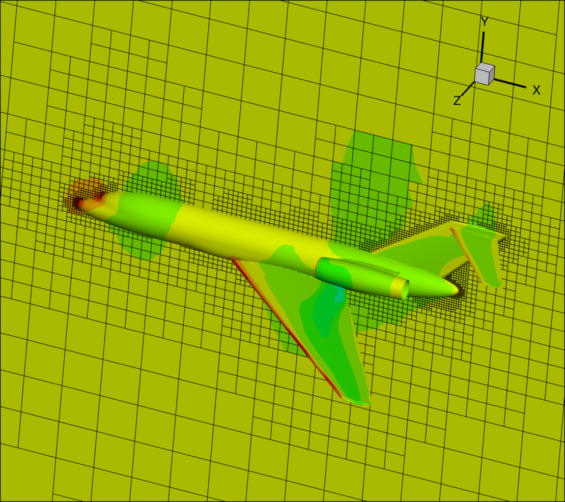
A sample graphic of the surface pressure made with Tecplot is shown below.
Figure 4.5 Business jet solution showing pressure with slice at y = 0 for
poweroff/m0.84a0.0b0.0 solution
The "RunControl" section of pyCart.json contains additional
information compared to previous examples for control of the mesh adaptation
settings. Here is a skeleton of the contents of that file.
{// The names of these two files have the obvious defaults."InputCntl":"inputs/input.cntl","AeroCsh":"inputs/aero.csh",// Phase settings and command-line options"RunControl":{// Run sequence"PhaseSequence":[0,1],"PhaseIters":[0,1000],// Overall settings"MPI":false,"nProc":8,"Adaptive":true,"flowCart":{...},"adjointCart":{...},// Parameters for autoInputs"autoInputs":{...},// Parameters for cubes"cubes":{...},"Adaptation":{...}},// Parameters for creating the mesh"Mesh":{...},// Describe the reference values and config."Config":{...},// Define the output functional"Functional":{...},// Requirements for the data book"DataBook":{...},// Report specifications"Report":{...},// RunMatrix description"RunMatrix":{"File":"inputs/matrix.csv","Keys":["Mach","alpha","beta","config","Label"],// Configuration name [default]"GroupPrefix":"poweroff",// Use the same mesh for all cases"GroupMesh":false}}
Note the very first two entries, "InputCntl" and "AeroCsh", specify
files in the inputs/ folder. Although this is not the default, it is a
good convention to keep all input template files in a separate folder. This
makes for a little less messy parent folder.
Most of the settings that have been replaced by ... in the preceding code
snippet are fairly straightforward, and the reader may refer to previous
examples. The two new sections are "Adaptation" and "Functional".
Let’s first look at the "Adaptation" function, which specifies mechanics
for mesh refinement.
"Adaptation":{// Number of adaptation cycles"n_adapt_cycles":[2,4],// Functional error tolerance"etol":0.000001,// Stop adapting when this number of cells is reached"max_nCells":50000000,// Number of flowCart iters on each new mesh// cycle 1 2 3 4 5 6 7 8 9 10 11+"ws_it":[200],// Growth in the number of cells// cycle 1 2 3 4 5 6 7+"mesh_growth":[1.5,1.5,2.0,2.0,2.0,2.0,2.5],// Adaptation type"apc":["p","a"]}
The n_adapt_cycles setting informs pyCart to perform 2 adaptation cycles in
phase 0 and a total of 4 (i.e., two additional cycles) in phase 1. As indicated
in the comments, ws_it specifies how many iterations to run on each
adaptation cycle, which is independent of phase. Similarly, mesh_growth
specifies the ratio of the size of the new mesh to the old mesh. Therefore, in
the four adaptation cycles, the mesh will grow by a total factor of
1.5*1.5*2.0*2.0, or 9.0. Finally, apc, specifies the type of cycle. An
"a" cycle is the standard type of mesh adaptation in which any cell may be
refined. In a "p" cycle, any cell which is the finest in the current mesh
may not be refined.
These "Adaptaion" settings are propagated to the Cart3D package of software
by editing lines of the aero.csh file.
The "Functional" section defines the scalar output function that is used to
drive mesh refinement. Roughly, the mesh refinement algorithm automatically
determines which cells will have the most significant effect on the output
function and refines enough of those to make the total mesh size grow by the
requested mesh_growth.
The key names (strings on the left-hand side of each : character) are just
used to define name each force for tracking purposes. The force parameter is
the axis number of the coefficient of interest (0 for the x axis, etc.),
the frame specifies either stability axes if 0 or body axes if 1, the
compID is the name or number of the component to use, and weight is the
weight with which that coefficient contributes to the overall functional. This
output functional gets defined in the input.cntl file. The relevant
lines are shown below.
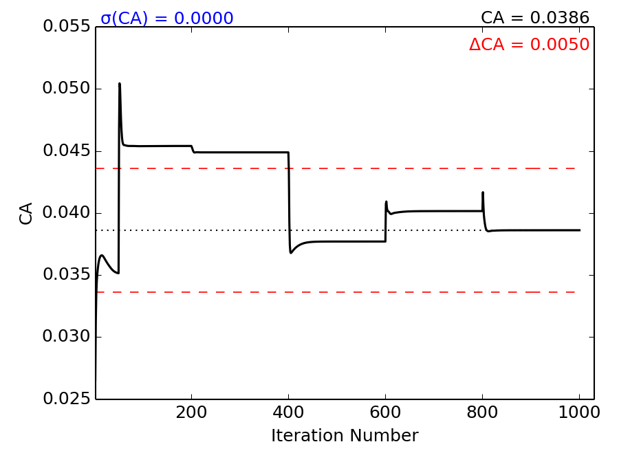
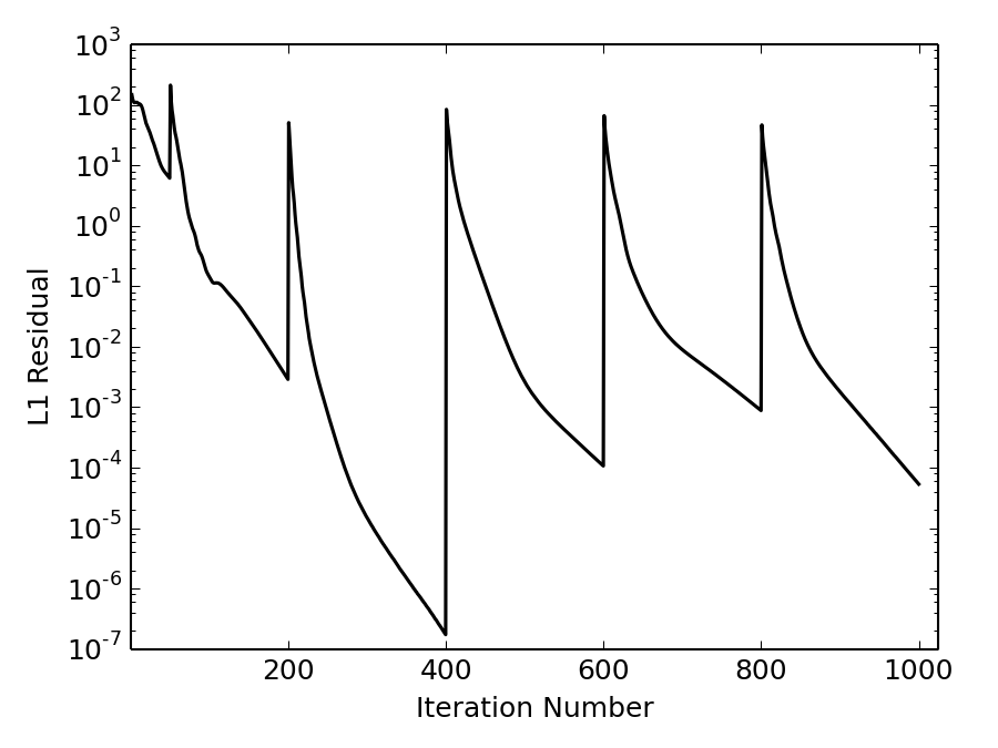
The following figures show some results from the poweroff/m0.82a0.0b0.0
case, which is the first case in the run matrix.
Plot of axial force coefficient, CA, for the component named “wing”
Plot of L1 global density residual
The residual plot very clearly shows how the residual converges to some degree
on each mesh adaptation cycle and then resets to a much higher level
immediately after each mesh refinement. The results of the previous cycle are
used as the initial conditions for the refined mesh (Cart3D refers to this as a
“warm start”), but the coarser solution projected onto the finer mesh does
result in a higher residual. The axial force coefficient clearly marks the
adaptation cycles as well. In this example, the value of CA appears to be
changing after each adaptation cycle, and so more mesh refinement would be
appropriate.