Python Wrappers¶

We have wrappers that allow the C+ Full Physics library to be used in Python.

The exact same doxygen documentation is available in Python using the standard Python help system, in particular you can issue a command such as help(AtmosphereOco).

Check the Python documentation generated using doxygen for information what classes are available through Python.

The wrappers are straight Python, but for interactive purposes use IPython, as well as the matplotlib and scipy libraries. If you aren’t familiar when them, you can take a look at their getting started guide.

Building¶

The Python bindings are not built by default, you need to explicitly request that the bindings be compiled. This is done by adding an option to the configuration line:

$ /path/to/source/configure --with-python-swig

You need to do a full install, not just a make all. This is because Python needs to see the libraries in a particular directory structure that gets created with the install. So you would build with:

$ make all && make install

Running¶

After building, you need to make sure that the Python path is set to point to the installed library. You can do this using the setup script installed in the install area:

$ source ./install/setup_fp_env.sh

Examples¶

First you will need to load the correct environmental variables then load a Python shell:

$ source ./install/setup_fp_env.sh
$ ipython --matplotlib auto

The easiest way to get started is by using a pre-existing Lua configuration:

In [1]: from full_physics import *
In [2]: from matplotlib.pylab import *
In [3]: conf = L2FpConfigurationLua('/path/to/existing_run/config.lua')

Add some information about getting the right enviromental variables made available.

Example 1 - Plotting Solar Spectrum¶

Get help on what conf is and can do:

In [3]: help(conf)

If you are using IPython, you can just use a ? after the object to get help:

In [3]: conf?

The solar model object is one of several spectrum effects, arbitrary operators on spectrum before instrument effects have been processed. It will probably be at index 0 of the spectrum effects list. Get help on what solar model is and can do:

In [4]: help(conf.forward_model.speceff_val(0, 0))

The second index above is the band index. Note that this is pretty much the same documentation as found in the Doxygen Documentation, or the Python Documentation but it can be convenient to do this in IPython without going to a browser.

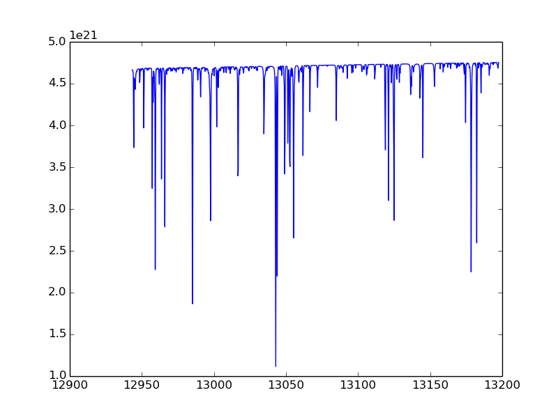
We can plot the solar model with a couple of short commands as follows:

In [5]: band = 0
In [6]: spec_dom = conf.forward_model.instrument.pixel_spectral_domain(band)
In [7]: solar_spec = conf.forward_model.speceff_val(0, band).solar_spectrum(spec_dom)
In [8]: plot(solar_spec.wavenumber, solar_spec.value)

Example 2 - Forward model without Jacobian¶

Run forward model and get radiances only for all the bands:

In [9]: r = conf.forward_model.radiance_all(True)

The boolean argument to radiance_all tells the code to skip Jacobian calculations.

Example 3 - Forward model with Jacobian¶

Run forward model and get radiance and Jacobian (takes longer to run):

In [10]: r = conf.forward_model.radiance_all()

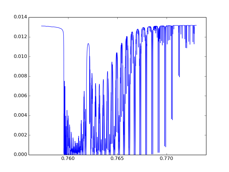
Example 4 - Radiative Transfer¶

Run just the radiative transfer w/o applying solar or instrument model:

In [11]: band = 0
In [12]: ils_hw = conf.forward_model.instrument.ils_half_width(band)
In [13]: spec_pix = conf.forward_model.instrument.pixel_spectral_domain(band)
In [14]: spec_samp = \
    conf.forward_model.spectrum_sampling.spectral_domain(band, spec_pix, ils_hw)
In [15]: rrt = conf.forward_model.radiative_transfer.reflectance(spec_samp, band, True)
In [16]: plot(rrt.spectral_domain.data, rrt.spectral_range.data)

We can also run the RT with Jacobian not disabled and then plot up a portion of the spectral data (first dim) for all state vector types:

In [17]: rrt = conf.forward_model.radiative_transfer.reflectance(spec_samp, band)
In [18]: jac = rrt.spectral_range.data_ad.jacobian
In [19]: matshow(jac[0:80, :], cmap=cm.jet)
In [20]: xlabel("State Index")
In [21]: ylabel("Spectral Point")

This shows that the Jacobian is dominated by one value:

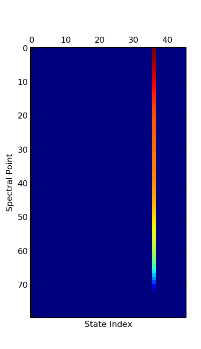
Look at vector and find largest one, and name of it:

In [22]: conf.forward_model.state_vector.state_vector_name[argmax(jac[0,:])]
Out[22]: 'Ground Lambertian A-Band Albedo Parm 2'

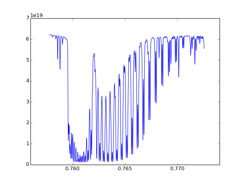
Example 5 - Apply Solar and Instrument Models¶

To apply the solar model and the instrument model along with other effects we would use the RT spectrum from the last example:

In [26]: rinst = conf.forward_model.apply_spectrum_corrections(rrt, band)
In [27]: plot(rinst.spectral_domain.data, rinst.spectral_range.data)

Example 6 - Use Generic Solver¶

DEPRECATED

Python SciPy comes with some generic solvers, including one based on the standard Fortran minpack routines. We have a version of the cost function that uses the more standard format of embedding the a priori values, a priori covariance matrix, and radiance uncertainty:

As an example of using this:

import scipy.optimize

cost_func = FmStandardFormatCostFunction(conf.forward_model(), \
        conf.spectral_window_apply().radiance(), \
        conf.spectral_window_apply().radiance_uncertainty(), \
        conf.initial_guess().apriori(), \
        conf.initial_guess().apriori_covariance())

x = conf.initial_guess().initial_guess()
cf = lambda x: cost_func.residual(x)
jf = lambda x: cost_func.jacobian(x)
yinitial = cf(conf.initial_guess().initial_guess())
print "Initial chisq: %f" % (sum(yinitial * yinitial)/ yinitial.size)
xsol, ier = scipy.optimize.leastsq(cf, x, Dfun=jf, maxfev=10)

if(ier < 0):
    print "An error occured"

ysol = cf(xsol)
print "Final chisq: %f" % (sum(ysol * ysol)/ ysol.size)

This print out:

Initial chisq: 131.571840
Final chisq: 18.775889

NOTE: This example only allows 10 evaluations of the cost function, and uses the default stopping criteria. This is really meant as a quick example, rather than saying this is a particularly good solver. Also, for C+ we were thinking of investigating the GSL. The GSL has python wrappers (PyGSL), and can be used as an alternative to the scipy solver. The standard Level 2 Full Physics solver gets a chisq of 0.614842 in 5 evaluations, so this example obviously needs some tuning to work for real.

More Advanced Example¶

DEPRECATED

The C+ interface exposed to Python has an interface centered around running the full physics retrieval. As we get feedback, we can extend this interface to be more useful in an investigative ipython environment. But you can also add your own layer of functionality on top of the lower level C+ interface, either as a quick prototype of a C+ interface change or instead of changing the C++.

As a concrete example, the interface to the radiative transfer holds things like the solar zenith angle, number of streams, etc. fixed since these don’t vary in the Level 2 Retrieval. But a very useful investigation would be to vary these parameters and see how they affect the Radiative Transfer results.

The ConfigurationHeritage interface in the earlier examples are tied to a particular run configuration file. But there is no reason that you need to create objects strictly from the run file, you can also use the more generic constructors of various classes, or modify objects after they have been created.

Continuing our example, here a wrapper class that sets up Lidort, the LRad polarization correction, and a model atmosphere based on the configuration file. You can then vary parameters such as the surface pressure, solar zenith angle, and number of streams. This example does not include the LSI speed up (since this example looks at a single wavelength), but you could include that is you wanted to for some reason.

We create a new class “RtExtraKnobs”. Save this in the file “rt_extra_knobs.py”. Note while you are developing code like this, you can repeatedly load updated versions by using the ipython “%run” command (once it is complete, you can just import it like any other module).

import full_physics as fp

class RtExtraKnobs:
    def __init__(self, fname="/groups/algorithm/python_tryout/sample_run/oco_l2.run"):
         conf = fp.ConfigurationHeritage(fname)
         self.conf = conf
         self.atm = conf.atmosphere()
         self.state_vector = conf.state_vector()
         self.level_1b = conf.level_1b()
         self.band = 0

    # Return radiance for single point for given solar zenith, pressure,
    # and number of streams
    def radiance(self, wn, sza, surface_press, nstream):
         try:
             self.atm.pressure().surface_pressure(surface_press)
             rt = self.__rt(sza, nstream)
             # Don't need log message for processing one point
             fp.FpLogger.turn_off_logger()
             return rt.radiance([wn], self.band)[0]
         finally:
             # Turn back on
             fp.FpLogger.turn_on_logger()

    # The relative azimuth needs to be modified because the convention used
    # in the OCO L1B1 file to to take both the solar and observation angles
    # as viewed from an observer standing in the FOV. LIDORT on the other
    # hand has the "follow the photons" convention. This results in a 180
    # degree change
    def __rel_azm(self, band):
         r = (180 + self.level_1b.sounding_azimuth(band)) - \
             self.level_1b.solar_azimuth(band)
         if(r >= 360): r = r - 360
         if(r < 0): r = r + 360
         return r

    # Get RT for a particular solar zenith angle and number of streams
    def __rt(self, solar_zenith, number_stream):
         band = self.band
         # Hardcode these for this example
         nbrdf_quadratures = 50
         nstoke = 3
         ss_corr = True
         delta_m_scaling = True
         uplooking = False
         # Value needed to be true for LRad
         get_rad_dif = True
         nmom = number_stream if(number_stream >= 4) else 4
         rt_lidort = fp.LidortDriver(self.atm, self.state_vector,
                                         [self.level_1b.stokes_coefficient(band)],
                                         [solar_zenith],
                                         [self.level_1b.sounding_zenith(band)],
                                         [self.__rel_azm(band)],
                                         number_stream, nmom, nbrdf_quadratures,
                                         nstoke, get_rad_dif, ss_corr,
                                         delta_m_scaling, uplooking)
         rt_lrad = fp.LRadDriver(rt_lidort, [solar_zenith],
                                     [self.level_1b.sounding_zenith(band)],
                                     [self.__rel_azm(band)])
         return rt_lrad

Once we have this module, we can use this in ipython to generate simple plots:

from rt_extra_knobs import *
rt = RtExtraKnobs()
wn = 13005.0
sza = 74.0
psurf = 96716.0
nstream = 16

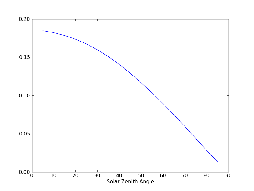
rad_by_sza = lambda x: rt.radiance(wn,x,psurf, nstream)
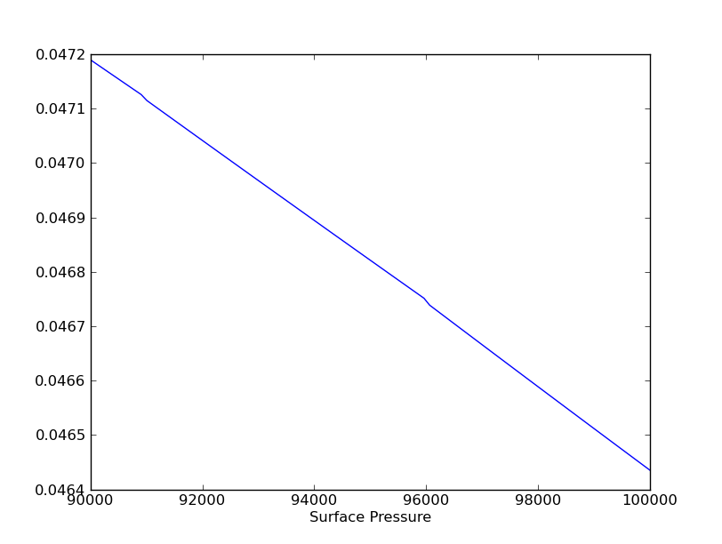
rad_by_psurf = lambda x: rt.radiance(wn,sza,x, nstream)
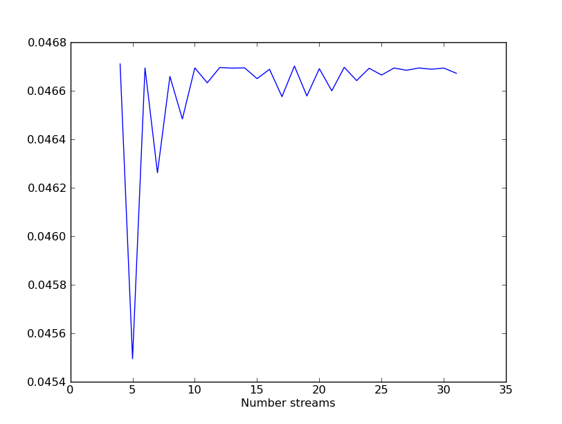
rad_by_nstream = lambda n: rt.radiance(wn,sza,psurf, int(n))

nstream_arr = r_[4:32]
plot(nstream_arr, map(rad_by_nstream, nstream_arr))
pylab.xlabel("Number streams")
sza_arr = r_[0:90:5]
plot(sza_arr, map(rad_by_sza, sza_arr))
pylab.xlabel("Solar Zenith Angle")
psurf_arr = r_[90000:100000:100j]
plot(psurf_arr, map(rad_by_psurf, psurf_arr))
pylab.xlabel("Surface Pressure")

Python Callback¶

To be documented - providing Python classes to be used in place of C+ (e.g., prototype a new LSI or solar model and test in retrieval).

RT Retrieval Framework documentation