CONTENTS

• New Features
• Summary of Input File Differences from Earlier Versions
• Limitations
• Known Problems

NEW FEATURES

This page lists new features in CFL3D Version 6. Because there is no Version 6 Manual, this page is very important because it supplements the Version 5 Manual by listing additional/changed features and capabilities of CFL3D. Of particular importance is the capability of "Keyword Driven Input," which is an optional section near the top of the standard CFL3D input file. See also the CFL3D Tutorial.

• Keyword Driven Input
  (click here for tables)
• Dynamic Memory Allocation
• Low Mach Number Preconditioning
• Additional Plot3d Output Options
• Specified Cl Option
• Block and Input File Splitter
• New Ronnie Input Options
• Error Code Files
• New Flux Limiter (iflim=4)
• New Normal Momentum BC 1006 for Inviscid Flows
• More General BC 2008, 2018, and 2028
• Specifying transition through BC 2014
• Imposing wall velocity through BC 2034
• Turbulence Data Input For 2000 Series BC's
• New BC 2016 for Suction and Blowing
• Solution Derivatives Via Complex Variables
• Entropy Fix for High Mach Number Conditions
• Turbulence Model Descriptions
• New inflow bc 2009, 2010, and 2019
• Specified Pressure Ratio 2103
• 2nd order temporal accuracy for turb models
• Graceful user-requested stop during program execution
• Source terms for non-inertial (rotating) reference frames
• New ihist option for force/moment convergence tracking
• DES and DDES capability
• Full Navier-Stokes capability
• Curvature correction capability for certain turbulence models
• Dacles-Mariani Rotation correction for SA model
• Keeping track of CL and CD on different bodies
• 2D and coarse movie output
• Variable CFLTAU (for time dependent calculations)
• Running-average Q-file (primarily for time dependant flows)
• More advanced running-average files (primarily for time dependant flows)
• Maintaining ambient turbulence levels without decay
• New unsteady aeroelasticity features
• Nonlinear Quadratic Constitutive Relation for use with Linear Models
• 3D Axisymmetric 2-plane cases with singular axis (under construction)
• Three- and four-equation transition models (under construction)
• Large eddy simulation (LES) capability (under construction)
• Method of Manufactured Solution for SA model (under construction)
• Ad-Hoc Separation Fix (under construction)
• New "sweeping jet" BC 2026 (under construction)
• Stress-Omega Full Reynolds Stress Models (under construction)

Keyword Driven Input

A number of users have requested that some standard constants, such as gamma (specific heat ratio), be specified via the input file. Because space is getting very tight in the input file, additional input is now accomodated via a "keyword driven" input. If used, the keyword driven input section must appear after the last input file name and before the case title. The keyword input section must begin with a line that has > in the first column (other characters may follow) and must end with a line that has < in the first column (other characters may follow).

The following example illustrates the use of the keyword input:

INPUT/OUTPUT FILES:
/net/aamber/scratch2/biedron/Multi/grid2.p3dunf
plot3dg.bin
plot3dq.bin
cfl3d.out
cfl3d.res
cfl3d.turres
cfl3d.blomax
cfl3d.out15
cfl3d.prout
cfl3d.out20
ovrlp.bin
patch.bin
restart.bin
>-- begin keyword-driven input section
gamma 1.30
pr    0.75
<-- end keyword-driven input section
Case Title
      MACH     ALPHA      BETA      REUE   TINF,DR     IALPH    IHSTRY
   0.95000   2.50000   0.00000 0.000E+00 393.00000         1         0

    etc...

In the example, additional characters are included after the required keyword section delimiters > and < in order to make the section stand out a bit more.

Note that the format is the keyword followed by the value you want the keyword variable to assume, without an equal sign. If a keyword variable is not specified, it will retain its default value. The following keywords are currently supported:

Note: the spelling of a keyword is important; if you misspell the name of the keyword, or use a keyword name that is not supported, the code will stop and print out the following message, following the offending keyword:

*** STOPPING: The keyword above is not supported. ***

Acknowledgment: Thanks to James O. Hager of Boeing Phantom Works, Long Beach, for suggesting and providing the model routines for keyword input

Return To Top

Dynamic Memory Allocation:

With the exception of MaGGiE, all codes in the version 6 release package have "dynamic" memory, though it is probably more precise to call them "self sizing", as most of the memory is allocated once and for all, and is not freed up after use. The self sizing ability is achieved by bringing the sizing codes (e.g. PRECFL3D for CFL3D, PRERONNIE for RONNIE) into the main code, and using pointers (a FORTRAN 77 extension) to allocate the memory determined by the sizing codes. Note that the sizing routines are still available as stand-alone codes, so that memory requirements can be determined before run time. This allows the user to determine which queue to submit the job to, or indeed if the job will fit on the Machine.

Acknowledgment: Thanks to Khaled S. Abdol-Hamid and Stephen J. Massey of Analytical Services and Materials, Inc., for showing how to implement dynamic memory allocation within FORTRAN 77

Return To Top

Low Mach Number Preconditioning:

Version 6 incorporates Jack Edwards' (North Carolina State University) implementation of the Weiss-Smith low Mach number preconditioning. This new capability is still undergoing evaluation, however preliminary assessment is that preconditioning is very helpful in obtaining convergence for low Mach number flows. Note: the preconditioner is really only effective for low freestream Mach numbers - in flows where the freestream Mach number is moderate, but with localized pockets of very low Mach number flow, this type of preconditioner has little effect. For Mach numbers above roughly 0.5 or so, the preconditioning loses its effectiveness, and can adversely affect convergence.

Sample Results

• 2D flow past a bump in a channel; the figures show the effect of preconditioning on the residual and lift coefficient convergence for a range of Mach numbers. Note: without preconditioning, the code will not even run below about Mach 0.2!
• Mach_0.70
• Mach_0.50
• Mach_0.20
• Mach_0.0001
• 3D flow past an ONERA M6 wing; the figures show the effect of preconditioning on the residual and drag coefficient convergence for a range of Mach numbers.
• Mach_0.84
• Mach_0.50
• Mach_0.10
• Mach_0.01
• Mach_0.0001

Keyword input of the parameters cprec, uref, and avn may be used to enable preconditioning.

The following definitions apply:

cprec

turns preconditioning fully on (cprec = 1.0), fully off (cprec = 0.0), or something in between (0.0 < cprec < 1.0). Setting cprec = 0.95 to 0.97 might be useful for stiffer low-speed problems

(default=0.0, i.e. NO preconditioning)

avn

multiplies the limiting velocity uref². Typically, avn should be around 1.0, but higher values may be needed for certain problems

(default=1.0)

uref

is the limiting velocity, nondimensionalized by the free-stream sound speed, meaning that it should be the same as the free-stream Mach number for most problems

(default=xmach)

The local "reference" velocity (vel) used in the preconditioned extensions is defined as follows:

vref2 = max[u**2 + v² + w², avn*uref²]

vel = min(a,sqrt(vref2))

vel = cprec*vel + (1.-cprec)*a, where a is the local sound speed

The basic preconditioning keyword input is simply:

>
cprec 1.0
<

Note: the default values of uref and avn will be used

Acknowledgment: Thanks to Jack Edwards of North Carolina State for the implementation of low Mach number preconditioning within CFL3D

Return To Top

Additional Plot3d Output Options:

The plot3d input parameter iptype has been expanded to include the following:

   iptype = 0...output q at grid points
           -1...output q at grid points, but use off-body wall parallel velocity
                instead of actual velocities at wall (which are zero),
                in order to more easily plot wall surface-restricted streamlines...
                should only be used in combination with nplot3d=-1
                (available after V6.6)
            1...output q cell centers
            2...turbulence data at cell centers, output in place of the
                standard plot3d q vector. (defaults in 2D are
                production-term,uw, uu, ww; defaults in 3D are
                production-term, uw, uu, ww Sk/eps)
            3...smin at cell centers
            4...eddy viscosity at cell centers
           -4...eddy viscosity at grid points (available after V6.4)
            5...cp at cell centers
           -5...cp at grid points
            6...p/pinf at cell centers
           -6...p/pinf at grid points
            7...turbulence index at walls (based on cell-center data); 
                only works for 3D cases (i2d=0) and
                should only be used in combination with nplot3d=-1...
                uses eqn 10 from Recherche Aerospatiale, Vol. 1, 1994, pp. 5-21,
                based on near-wall eddy viscosity translated to 
                Spalart-Allmaras variable form... this formula is appropriate
                for S-A, but only an approximate (crude) indicator for other models
                (available after V6.6)

• general rule: iptype <= 0 gives grid point data, iptype > 0 gives cell-center or cell-face-center data
• If nplot3d = -1, then the code will look for any surfaces that have bc types 1004, 2004 or 1005 (i.e. solid surfaces), and output those to the specified plot3d files. This can provide an excellent means of determining if all solid surfaces are specified correctly in the boundary condition section.
• if nplot3d = -1, one line of plot3d input data MUST appear in the plot3d data section near the bottom of the input file. In this one line of plot3d data, only the value of iptype is used; all other values are ignored and may be set to zero. Note that this is different than the procedure in Version 5, where nplot3d = -1 expected NO lines of plot3d input.

• if cell center data is requested (iptype > 0) and nplot3d = -1, then cell FACE CENTER data is output for cell faces lying on solid surfaces
• if nprint = -1, the same comments apply as for nplot3d < 0, but note that in the print out section, only iptype = 0 or 1 are valid types for print out

Return To Top

Specified Cl Option:

It may sometimes be desired to obtain a solution for a fixed or known lift coefficient. In that case alpha is unknown and must be obtained as part of the solution. CFL3D has had an option for this for a while, but the method has been UPDATED (for Version 6.2 and later). One major change with the new method is that the entire flowfield's velocity vectors are now rotated when the angle of attack is updated. Also, in the new method, the updating of angle of attack generally occurs more often (default is every iteration), and the change allowed each time step is smaller. The old method for doing specified CL is no longer available.

Keyword input of the parameters cltarg, rlxalph, icycupdt, and dalim may be used to enable the specified Cl option. (Keywords resupdt and dcldal were used for the old method, and are no longer available.)

The following definitions apply

cltarg

the desired lift coefficient

(default=99999.0, for which the spcified Cl option is OFF)

rlxalph

relaxation factor used to update angle of attack; it multiplies the difference between the current CL and the target CL (cltarg).

(default=1., meaning no under- or over-relaxation)

icycupdt

number of cycles between alpha updates (.le. 0 means alpha will not be updated).

(default=1, update every iteration)

dalim

limit of alpha change (deg.) per update

(default = 0.2, should be fine for most cases)

alpha

(NOT a keyword input) the initial value of alpha from which to start the solution. NOTE: if restarting, the value of alpha from the restart file is used, and the input value is ignored

To utilize the specified Cl option, generally only cltarg needs to be set. For some cases, however, the default options may result in a limit-cycle oscillation in CL (and alpha). When this occurs, one strategy is to adjust (usually lower) rlxalph. Another strategy is to update every n iterations rather than every iteration, by increasing icycupdt.

NOTE: the following alpha-iteration parameter is hard-coded in subroutine newalpha; the user may want/need to alter this parameter:

ioalph

if > 0, output alpha history to cfl3d.alpha (set at 1). Note that in cfl3d.alpha, past alpha history is not preserved after a a restart.

The final alpha (and Cl) will also appear at the top of the standard convergence history file.

Acknowledgment: Thanks to Steve Allmaras of Boeing-Seattle for providing the coding of this feature.

Return To Top

Block and Input File Splitter:

Instructions on how to use the block splitter can be found in Block Splitter

To insure that split grids produced the same results as the original unsplit grids when fully converged, two modifications were made to previous versions of CFL3D:

• A new flux limiter, number 4, was introduced. This new limiter is a modified version of the heretofor recommended limiter number 3. Both versions are tuned to the k=1/3 ("third order" upwind) scheme. The new number 4 is similar to the old number 3, but with a cutoff parameter based on the total number of cells, rather than block dimensions. As a grid is split, the total number of cells remains fixed, but of course block dimensions do not. Use iflim=4 whenever a limiter is required for k=1/3. The graphic shows the effect of the choice of the k=1/3 limiter on a 2D airfoil solution:

  • compare limiters

  Note 1: iflim=3 and iflim=4 will generally give slightly different results even for single block grids, since iflim=3 actually bases the cutoff parameter on the dimension in each direction for which the limiter is applied; iflim=4 uses a cutoff parameter that is isotropic.

  Note 2: limiters iflim=1 and iflim=2 (and iflim=0, no limiting) are uneffected by block splitting when fully converged.

• Correct cell volumes at 1-1 interfaces are now used. The volumes at block interfaces are used in the viscous flux routines; in previous versions of CFL3D, these interface volumes were simply extrapolated from interior cells. If a block is split, what was an interior volume now lies on a block interface. How that volume is treated can affect the solution, depending on how highly streched that grid is in that region. Version 6 uses the exact interface volumes at 1-1 interfaces, so that the same results can be obtained before and after splitting. EXCEPTION: The Menter SST turbulence model (ivisc=7) uses a blending function that is not split exactly. Very slight differences may be observed if a block is split in a region of strong gradients when using ivisc=7. The graphic shows the effect of the treatment of cell volumes at 1-1 interfaces.

  • compare v5/v6

The convergence rate may be expected to deteriorate as blocks are split finer and finer since the implict nature of the scheme extends only over points that lie in the same block. However, in many cases, this deterioration may be quite small, as evidenced in the 2D airfoil case above. The following graphic shows the convergence rate for a 3D ONERA M6 wing with approximately 1 million points, with 1 zone (289x65x49), 96 zones (each 37x17x17) and 216 zones (each 17x17x17), with remarkably little deterioration in convergence of either the residual or the drag:

• split convergence

Return To Top

New Ronnie Input Options:

The latest version of the ronnie patched-grid code is included with this release. In this release, ronnie is actually "created" out of the dynamic patching routines from cfl3d, plus a few driver routines. This avoids duplication of essentially identical code, and assures complete consistance between stand-alone patching and dynamic patching. In addition, it opens up the opportunity in ronnie to shift and rotate grids before they are patched. One application of this is to the simulation of 2D cascade flows, where periodicity can be obtained for grids which don't match 1-1 on the periodic boundaries. What's new:

• Ronnie now supports 3 input file styles. The first new style was added to allow user-specified search range on the "from" side - this should overcome some difficult search problems at the expense of additional user input. The second new style is a result of the merging of ronnie and cfl3d's dynamic patching routines.
• Ronnie has been modified to increase robustness when attempting to determine interpolation data on coarser levels. In the past, the search routines would sometimes fail on coarser levels, despite having successfully determined all the corresponding stencils on a finer level. Now, if the routines initially fail on a coarser level, ronnie will set coarser level stencils by collocating fine grid data.
• The file names created when diagnostic plot3d output is generated (either automatically or by setting ifit < 0) have been changed. The old file names where fort.xx, where xx is the interpolation number. The new file names are denoted by patch_p3d.xx. The new names avoid the limit on some systems of creating a file past fort.99.

The differences between the old and new styles are described below:

OLD Style:

INPUT/OUTPUT FILES
shockg.bin_sngl
ronnie.out
patch.bin
Title
.
.
.

New Style:

INPUT/OUTPUT FILES
shockg.bin_sngl
ronnie.out
patch.bin
IOFLAG  ITRACE
1       -1
Title
.
.
.

where:

ioflag

= 1 allows new input format (1) as indicated below

= 2 allows new input format (2) as indicated below

= 0 for the old input format (where all the "from" blocks are on one line)

itrace

= -1....no tracing

= 0....save trace from last cell only

= +1....save trace from all cells searched so far (may give big file!)

itrace .ne. -1 primarily intended for the code developer

Old Style:

 INT    TO   XIE1  XIE2   ETA1   ETA2   NFB  FROM  FROM  FROM  FROM...
   1  0112      0     0      0      0     1  0411
   2  0212      0     0      0      0     1  0411 
   3  0312      1   113      0      0     1  0411
   4  0312    113   245      0      0     1  0411
   5  0312    245   337      0      0     1  0411
   6  0411      0     0      0      0     3  0112  0212  0312

New Style (1):

 INT    TO   XIE1  XIE2   ETA1   ETA2   NFB (one per int)
      FROM   XIE1  XIE2   ETA1   ETA2       (repeat nfb times for each int)
   1  0112      0     0      0      0     1  
      0411      0     0      0      0
   2  0212      0     0      0      0     1
      0411      0     0      0      0
   3  0312      1   113      0      0     1
      0411      0     0      0      0
   4  0312    113   245      0      0     1
      0411      0     0      0      0
   5  0312    245   337      0      0     1
      0411      0     0      0      0
   6  0411      0     0      0      0     3  
      0112      0     0      0      0
      0212      1    21      1     97
      0312      0     0      0      0

New Style (2) (See Version 5 user manual, Chapter 3, LT43-LT45):

   INT    TO     XIE1     XIE2     ETA1     ETA2      NFB
     1  0112        0        0        0        0        1
        FROM     XIE1     XIE2     ETA1     ETA2    FACTJ    FACTK
        0411        0        0        0        0    0.000    0.000
                   DX       DY       DZ   DTHETX   DTHETY   DTHETZ
                0.000    0.000    0.000    0.000    0.000    0.000
   INT    TO     XIE1     XIE2     ETA1     ETA2      NFB
     2  0212        0        0        0        0        1
        FROM     XIE1     XIE2     ETA1     ETA2    FACTJ    FACTK
        0411        0        0        0        0    0.000    0.000
                   DX       DY       DZ   DTHETX   DTHETY   DTHETZ
                0.000    0.000    0.000    0.000    0.000    0.000
   INT    TO     XIE1     XIE2     ETA1     ETA2      NFB
     3  0312      113      245        0        0        1
        FROM     XIE1     XIE2     ETA1     ETA2    FACTJ    FACTK
        0411        0        0        0        0    0.000    0.000
                   DX       DY       DZ   DTHETX   DTHETY   DTHETZ
                0.000    0.000    0.000    0.000    0.000    0.000
   INT    TO     XIE1     XIE2     ETA1     ETA2      NFB
     4  0312      113      245        0        0        1
        FROM     XIE1     XIE2     ETA1     ETA2    FACTJ    FACTK
        0411        0        0        0        0    0.000    0.000
                   DX       DY       DZ   DTHETX   DTHETY   DTHETZ
                0.000    0.000    0.000    0.000    0.000    0.000
   INT    TO     XIE1     XIE2     ETA1     ETA2      NFB
     5  0312      245      337        0        0        1
        FROM     XIE1     XIE2     ETA1     ETA2    FACTJ    FACTK
        0411        0        0        0        0    0.000    0.000
                   DX       DY       DZ   DTHETX   DTHETY   DTHETZ
                0.000    0.000    0.000    0.000    0.000    0.000
   INT    TO     XIE1     XIE2     ETA1     ETA2      NFB
     6  0411        0        0        0        0        3
        FROM     XIE1     XIE2     ETA1     ETA2    FACTJ    FACTK
        0112        0        0        0        0    0.000    0.000
                   DX       DY       DZ   DTHETX   DTHETY   DTHETZ
                0.000    0.000    0.000    0.000    0.000    0.000
        FROM     XIE1     XIE2     ETA1     ETA2    FACTJ    FACTK
        0212        1       21        1       97    0.000    0.000
                   DX       DY       DZ   DTHETX   DTHETY   DTHETZ
                0.000    0.000    0.000    0.000    0.000    0.000
        FROM     XIE1     XIE2     ETA1     ETA2    FACTJ    FACTK
        0312        0        0        0        0    0.000    0.000
                   DX       DY       DZ   DTHETX   DTHETY   DTHETZ
                0.000    0.000    0.000    0.000    0.000    0.000

Return To Top

Error Code Files:

For ease of integration of CFL3D and its related codes into automated design packages, an error code file is created with the nomenclature code.error (e.g. cfl3d.error or splitter.error). The standard format for these error files is

error code:

numerical error code in written in i3 format (0 - normal, < 0 - abnormal)

termination status

description of error if termination status is abnormal

examples:

• program completes normally

    error code:
     0
    execution terminated normally

• abnormal termination

    error code:
    -1
    abnormal termination:
    input file error

Currently, CFL3D, PRECFL3D, RONNIE, PRERONNIE and SPLITTER all generate error code files

Return To Top

New Normal Momentum BC 1006 for Inviscid Flows:

BC type 1006 (which is not documented in the printed manual) is included in Version 6. This boundary condition for inviscid walls uses the normal momentum equation to obtain the wall pressure. This helps avoid "kinks" in the solution (such as in Mach contours) near slip-walls which often occur using bc1005

Return To Top

More General BC 2008, 2018, and 2028:

BC types 2008, 2018, and 2028 (which are not documented in the printed manual) are included in Version 6. These boundary conditions are for various types of "specified subsonic inflow", useful for inflow into ducts or channels where flow variables are known.

------------

BC2008: the user specifies density and velocity components, and pressure is extrapolated from the interior. The standard required input data is:

ndata = 4

with

rho/rho_ref, u/a_ref, v/a_ref, w/a_ref

specified via the input file, while pressure is extrapolated from the interior of the domain. This BC is appropriate as a general subsonic-inflow BC. Note that "ref" refers to "reference" quantities.

Important: previous usage of bc2008 was ndata=5, with u/a_inf, v/a_inf, w/a_inf, turb1 and turb2 specified; this usage is not correct for Version 6; Version 5 still supports the old usage

------------

BC2018 (new for Version 6.2): the user specifies temperature and momentum components, and pressure is extrapolated from the interior. The standard required input data is:

ndata = 4

with

T/T_ref, rho*u/(rho_ref*a_ref), rho*v/(rho_ref*a_ref), rho*w/(rho_ref*a_ref)

specified via the input file, while pressure is extrapolated from the interior of the domain (it uses this pressure along with the specified temperature to determine the density). This BC is appropriate as a general subsonic-inflow BC. Note that "ref" refers to "reference" quantities.

------------

BC2028 (new for Version 6.2): the user specifies frequency and maximum momentum components; density and pressure are both extrapolated from the interior. The standard required input data is:

ndata = 4

with

freq*l_ref/a_ref, (rho*u)_max/(rho_ref*a_ref), (rho*v)_max/(rho_ref*a_ref), (rho*w)_max/(rho_ref*a_ref)

specified via the input file, while density and pressure are extrapolated from the interior of the domain. Note that "ref" refers to "reference" quantities. The velocity profiles alternate between suction and blowing in a sinusoidal fashion via, for example, (rho*u)_max/rho*cos(2*pi*freq*t) for time-accurate flow. (If the case is not run time-accurately, then the momentum components will remain fixed.)

------------

For each of 2008, 2018, and 2028, with ndata=4 turbulence data is set from freestream conditions. But see also the section Turbulence Data Input For 2000 Series BC's describing an enhancement to all 2000 series BCs for including turbulence data in the input.

Return To Top

Imposing wall velocity through BC 2034:

New to versions beyond Version 6.7 is the capability to impose a wall velocity via a BC type (for an adiabatic solid wall). This BC is the same as BC2004, except that it accepts the keywords: uub_2034, vvb_2034, wwb_2034, or vvb_xaxisrot2034, which modify the wall velocity (these are imposed velocities nondimensionalized by the reference speed of sound). The uub_2034, vvb_2034, and wwb_2034 are prescribed u, v, and w velocities, respectively. The vvb_xaxisrot2034 is an imposed rotational velocity about the x-axis. The standard required input data is the same as for BC2004.

Return To Top

Specifying transition through BC 2014:

New to Version 6.2 is the capability to specify transition location through a BC type, rather than through ilamlo, ilamhi, etc. This type, BC 2014, is not documented in the printed manual. The main advantage to the new method is that you are no longer limited to having only one laminar region per zone. BC 2014 is exactly the same as BC 2004 (viscous surface), described in the manual, except that it also forces the specified region to be laminar by zeroing out the turbulence production term. It only works for ivisc greater than 3.

The standard required input data is:

ndata = 3

with

Twtype, Cq, Index

specified via the input file. Note that this is different from BC 2004 in that BC 2004 only uses 2 items of input data. The Twtype and Cq parameters here are the same as the 2 inputs required for BC 2004 (see manual). The additional Index parameter for BC 2014 represents the index range normal to the surface over which the laminar region is to extend. Setting Index=0 defaults to the entire normal index range. For example, say that a laminar viscous wall patch (adiabatic, no blowing/suction) is desired on a jmin surface from i=17-33 and k=65-129, over all j-indices normal to the surface. The input would look like:

J0:   GRID   SEGMENT    BCTYPE      ISTA      IEND      KSTA      KEND     NDATA
         1         1      2014        17        33        65       129         3
    TWTYPE        CQ     INDEX
        0.        0.         0

J0:   GRID   SEGMENT    BCTYPE      ISTA      IEND      KSTA      KEND     NDATA
         1         1      2014        17        33        65       129         3
    TWTYPE        CQ     INDEX
        0.        0.        25

JDIM: GRID   SEGMENT    BCTYPE      ISTA      IEND      KSTA      KEND     NDATA
         1         1      2014        17        33        65       129         3
    TWTYPE        CQ     INDEX
        0.        0.        25

Unless there are walls at both jmin and jmax, usually one would probably want to use the first method above (Index=0). Note that the old ilamlo, ilamhi, etc method for prescribing laminar regions still works. In fact (although not recommended), both methods can be used simultaneously. The laminar regions are the unions of the regions defined by ilamlo, ilamhi, etc. and those defined by the 2014 boundary condition. In general, however, we recommend doing either one method or the other, to avoid confusion.

Return To Top

Turbulence Data Input For 2000 Series BC's:

The following 2000 series bc's will now allow the user to input data for the turbulence field equations: 2003, 2007, 2008, 2018, 2028, 2009, 2010, and 2019 (note: standard data specification for 2008 has changed for Version 6, see above). The standard values of ndata for bc's 2003, 2007, 2008, 2018, 2028, 2009, 2010, and 2019 are 5, 5, 4, 4, 4, 4, and 2 respectively. If these standard ndata are increased by 1 (for 1 equation turbulence models) or 2 (for 2 equation turbulence models), then the additional data is used to set the boundary conditions for the turbulence equations (Note: this is not applicable to Baldwin-Lomax). If the standard ndata is used, then the boundary condition for the turbulence data is the same as before: for 2003, 2009, 2010, and 2019, the turbulence variables are set to freestream values if inflow, or extrapolated from the interior if outflow; for 2007, 2008, 2018, or 2028, the turbulence variables are set to freestream values.

Note: the additional turbulence data must be input as nondimensional, appropriate for the particular turbulence model in use. See Appendix H of the Version 5 manual for details of the turbulence models and the appropriate nondimensionalizations.

As an example, consider bc2008, and assume that the 2-equation SST model is used (ivisc=7):

J0:   GRID   SEGMENT    BCTYPE      ISTA      IEND      KSTA      KEND     NDATA
         1         1      2008         0         0         0         0         6
RHO/RHOINF    U/AINF    V/AINF    W/AINF     TURB1     TURB2
     1.000      0.95     0.000     0.000     1.e-6     9.e-9

These new turbulence data treatment also supports data read in from files, if ndata is negative.

Return To Top

New BC 2016 for Suction and Blowing:

BC 2016 is an extension of BC 2004, offering additional options for the prescription of mass flow through a solid boundary. The structural forms of the two routines are the same and so are their interfaces with the main code. BC 2016 may be used in place of BC 2004 when the additional options are needed. This boundary condition is implemented into official versions of CFL3D only after V6.3. BC 2016 enables two modes of operation:

1) rfreq .ge. 0.0: A steady component of mass flow is prescribed plus an unsteady component that varies sinusoidally in time. (If the case is not run time-accurately or if rfreq=0, then the mass flow rate will remain fixed at cq or at the rate it last was when time-accurate time stepping was on.)

2) rfreq .lt. 0.0: A constant rate of change in mass flow from zero to a terminal (constant) value is prescribed. (If the case is not run time-accurately, then the mass flow rate will remain fixed at zero or at the rate it last was when time-accurate time stepping was on.)

BC 2016 requires a total of seven pieces of auxiliary data:

• twtype (same definition as for BC 2004)
• cq (same definition as for BC 2004)

  -if rfreq .ge. 0.0, then cq is the coefficient of a steady component of mass flow

  -if rfreq .lt. 0.0, then cq is the terminal value of a mass flow coefficient that is ramped from zero to cq

• cqu

  -if rfreq .ge. 0.0, then cqu is the coefficient of an unsteady component of mass flow (the unsteady component is sinusoidal in time, and the total mass flow is the sum of the steady and unsteady components)

  -if rfreq .lt. 0.0, then cqu is the constant rate of change with respect to nondimensional time in total mass flow from zero to cq

• sjetx, sjety, sjetz are the direction numbers of the blowing/suction in the x, y, and z directions, respectively. For example, if sjetx=1 and sjety=sjetz=0, then the blowing/suction will act in the x-direction. If sjetx=0.5, sjety=0, and sjetz=0.5, then the blowing/suction will act at a 45 deg. angle in the x-z plane. The direction numbers do not need to be normalized. If all three direction numbers are zero, then the mass flow will default to be normal to the surface, and the sign convention is the same as the sign convention for cq in BC 2004.
• rfreq (Note that rfreq=freq*lref/aref, where freq is in Hz, lref is the reference length, and aref is the reference speed of sound.)

  -if rfreq .ge. 0.0, then rfreq is the reduced frequency of an unsteady component of mass flow, where the unsteady component is cqu*sin(2*pi*rfreq*time)

  -if rfreq .lt. 0.0, then the absolute value of rfreq does not matter, and the total mass flow coefficient is equal to cqu*time until the value of cq is reached, at which point the mass flow remains constant with a coefficient of cq.

Acknowledgment: Thanks to Hal Carlson of Clear Science Corp. for coding this boundary condition.

Return To Top

Solution Derivatives Via Complex Variables

The complex variable approach for generating solution derivatives of numerical schemes is not a new idea, having been proposed in 1967 by Lyness and Lyness and Moler. However, it did not see much use until it was revived by Squire and Trapp in 1998 ("Using Complex Variables to Estimate Derivatives of Real Functions" SIAM Review, Vol 10, No. 1, March 1998, pp.110-112). Kyle Anderson popularized the method at NASA Langley ("Sensitivity Analysis for the Navier-Stokes Equations on Unstructured Meshes Using Complex Variables.", AIAA Paper No. 99-3294, June 1999).

The method is based on the Taylor series expansion of a complex function

f(x+ih) = f(x) +ihf'(x) -0.5h²f''(x) + O(ih³)

so that equating the imaginary parts on the left and right hand sides gives

f'(x) = Im[f(x+ih)]/h + O(h²)

The derivative is subject to a truncation error on the order of the square of the step size, but, quite importantly, is not obtained by differences of two nearly identical numbers as is done in finite differences. Thus, unlike finite differences, the step size h can be made as small as desired without subtractive errors (i.e. numerical precision) ever swamping the truncation error. A step size of 1.e-6 is generally quite sufficient.

Although not available at the time that CFL3D was converted to complex variables, Joaquim Martins at Stanford University has developed a script to automate the conversion of a FORTRAN 90 code to complex variables.

A complex version of the parallel code can be generated by typing:

make cfl3dcmplx_mpi

in the build directory. Alternatively, a complex sequential version of the code can be generated by typing:

make cfl3dcmplx_seq

Because the entire code is rendered complex, any real data that comes into the code can potentially be an independent variable with respect to which derivatives of the solution can be obtained. All that is required is to simply give that variable a small complex component. The following variables are already implemented into the code, with the input variable for the appropriate "h" step given in parentheses, and are accessable via Keyword input:

• Mach number (xmach_img)
• unit Reynolds number (reue_img)
• angle of attack (alpha_img)
• yaw angle (beta_img)
• free stream temperature (tinf_img)
• geometry (geom_img)
• rotation rate about the x-axis (xrotrate_img)
• rotation rate about the y-axis (yrotrate_img)
• rotation rate about the z-axis (xrotrate_img)

Note that for geometrical derivatives, the value of geom_img must correspond to the step size used to generate the complex-valued grid. To split a complex-valued grid, use splittercmplx (see Block Splitter). The resulting derivatives of Cl, Cd,Cm, etc are output to the file cfl3d.sd_res - this is a file similar to the usual CFL3D convergence history file cfl3d.res for the solution convergence. For example, to determine the derivatives with respect to angle of attack, start with a standard CFL3D input file set up for the angle of attack of interest, and then add the Keyword input:

>
alpha_img 1.e-8
<

The complex-valued code will require twice the memory and approximately three times the CPU time of the real-valued code. Derivatives can be obtained by central differences for twice the CPU time. However, finite differences are subject to large truncation error if the step size is too small and large subtractive error if the step size is too small, so factoring in the "trial and error" of step size choice can easily make the complex-variable approach very competetive, CPU-wise. The following figures illustrate this.

The first figure shows the convergence of a 32 block grid for the ONERA M6, using roughly 10⁶ grid points. Convergence is quite acceptable, with the drag varying less than 1 count (0.0001) after 200 coarse level + 200 medium level + 500 fine level iterations. However, the residual does "hang" on the level of roughly 10^-9. Evaluating the derivative of drag with respect to angle of attack by calculating two different solutions with small differences in angle of attack and using finite differences with various step sizes leads to wildly different, mostly garbage, results. For comaprison, the derivative computed using the complex code converges as well as the function. Total "cost" of the single complex derivative calculation was 3 times the cost of a standard solution. For the finite derivative result, a total of 6 runs were made, but each was run roughly twice as long on the fine level in order to try and get decent derivatives. This was a "real-world" scenario, in that the initial choice of finite difference step size was chosen as 10^-6 since that had worked quite well in other cases.

• solution convergence
• derivative convergence

• complex-variable vs. ADIFOR convergence

IMPORTANT NOTE #1: restart files are NOT compatable between the "regular" version of CFL3D and the complex version.

IMPORTANT NOTE #2: As of March, 2007, the Intel Version 9 compiler has major problems with complex cases in CFL3D. If you use Intel, consider compiling with a different version.

Return To Top

Entropy Fix for High Mach Number Conditions

In an attempt to increase the robustness of the code at high Mach numbers, an option to include an "entropy fix" has been added to Roe's scheme (ifds=1). This ammounts to a modification of the eigenvalues in instances where they approach zero, and has the effect of making the scheme more dissipative. The particular version of the entropy fix is that described in NASA TP-2953:

with the slight difference that here, u,v,w are taken as the covariant velocities, rather than the contravariant velocities. The subscript i indicates the i-th eigenvalue, and c is the sound speed. Lamdas without overbars are the unmodified eigenvalues from Roe's scheme. The parameter epsilon is input as the Keyword input epsa_r. Typical values are in the range of 0.0 to 0.4, with epsa_r = 0. corresponding to the original Roe scheme; epsa_r = 0.3 is a good general choice when an entropy fix is required.

NOTE: For high Mach numbers, the entropy fix should be used in conjunction with the 5x5 block inversion option (idiag = 0).

Sample Results

• 2D calculations for flow past a ramp of 34 degrees. A value of epsa_r = 0.3, in conjunction with idiag=0, was used; the standard Roe scheme diverges, even with idiag=0.
• convergence
• pressure

• 2D calculations for flow around an RAE 2822 for a range of Mach numbers. Note that at Mach 10, the standard Roe scheme diverges.
• convergence, Mach 10.0
• convergence, Mach 0.75
• convergence, Mach 0.30

The Mach 0.30 and Mach 0.75 cases are shown to assess the effect on the somputed forces due to the extra dissipation, since these are cases that run without the entropy fix. The following table presents the lift and drag values obtained on a series of 3 meshes, with Richardson extrapolation to zero cell size, for epsa_r = 0 and epsa_r = 0.3. At least for these cases, little effect on the lift and drag was seen when employing the entropy fix.

Acknowledgment: Thanks to Peter Gnoffo of NASA-Langley Research Center for providing the LAURA implementation of this feature, which provided the basis for the implementation in CFL3D Version 6.

Return To Top

Turbulence Model Descriptions

The following table summarizes the turbulence models in CFL3D, including the differences between Version 5 and Version 6. In the table, ivisc refers to the parameter in the CFL3D input file that controls the turbulence model choice.

Notes:

• Baldwin-Lomax #2 and #3 is not recommended because it is not a field-equation model and hence has dependence on the grid structure; it is particularly ill-suited for multiple-zone grids.
• Baldwin-Barth #4 is not recommended because it is ill-conditioned near the edge of boundary layers and can yield non-physical behavior there (see J. Fluids Eng., Vol. 119, No. 12, 1997, p.876-884).
• Model #9 is the same as model #13 with no nonlinear terms included in the tau_ij's in the RHS of the Navier-Stokes equations. Similarly, model #8 represents a linear version of #14. These linear versions are not recommended in general, because they are not complete models (they were originally intended for use only to initiate steady-state calculations for models #13 and #14).
• The EASM models #11 and #12 are not recommended because they utilize "constant g", which is not believed to be as accurate for many flows as the EASM method which solves a cubic equation and hence properly accounts for the production-to-dissipation-rate ratio in the flow (see AIAA J., Vol. 38, No. 8, 2000, p. 1394-1402).
• The k-enstrophy model #15 is a new turbulence model addition effective Version 6.4 and later. The original reference is: AIAA J., Vol. 36, No. 10, 1998, p.1825-1833.
• The k-kL-MEAH2015 model #16 is a new turbulence model addition effective Version 6.7 and later. The original reference is: Int J Aerospace Eng, Vol. 2015, Article ID 987682. (Note there is missing information in the paper, and some minor modifications have also been made. A more complete description can be found on http://turbmodels.larc.nasa.gov.
• All models, particularly k-epsilon and k-enstrophy versions, sometimes fail to go turbulent on their own where desired. It is recommended that the user always check resulting vist3d (eddy viscosity) levels output by the code, to insure that turbulence has tripped. If a model fails to trip, we recommend either restarting from a different converged model, or, if starting from scratch, freezing the model to its initialized levels (using Keyword input nfreeze) until the mean flowfield is advanced enough for turbulence to sustain itself.
• K-epsilon models (including Abid and EASM k-epsilon) are generally not recommended for use with adverse-pressure-gradient wall-bounded flows. Most k-epsilon types of models are known to yield generally very poor results in such situations (see, for example, discussions on this point in D. C. Wilcox, "Turbulence Modeling for CFD," 2nd Ed., DCW Industries, La Canada, CA, 1998).
• When running turbulence models, the grid should be fine enough such that the minimum spacing near the walls yield a y+ value of order 1. Some of the turbulence models are more sensitive to this precise value than others. The y+ levels are printed out near the bottom of the CFL3D standard output file. Wall functions can be employed when grids have larger minimum spacing (by setting ivisc in the input file to a negative number), but the wall function approach is strictly an incorrect approximation for separated flows, and is not recommended in general.
• The EASM models typically tend to be less robust than other turbulence models. The most robust models are usually SA and SST (ivisc=5 and 7).
• For the k-enstrophy model, the original paper (AIAA J., Vol. 36, No. 10, 1998, p.1825-1833) stated that the parameter beta8 could be taken as zero (as opposed to its standard value of 2.3) to avoid numerical problems. Currently the default in CFL3D is beta8=0. This may be changed to 2.3 by setting the Keyword input ibeta8kzeta to 1. Also, note that for the k-enstrophy model the default value for Keyword input tur1cut is -1, which means that the enstrophy variable is not updated at all when it tries to drop below tur1cutlev.
• There are many code input options related to turbulence models available as Keyword input. These include 2nd order spatial advection (as opposed to 1st order), different order of temporal accuracy from the mean flow, and the option to specify different freesteam turbulence levels. The defaults in the code have been determined as generally valid or useful for most applications. In many cases, a trade-off between accuracy and robustness had to be made. Many of the defaults were chosen simply to preserve backward compatability with earlier versions of the code.
• When using Keyword input for ikoprod or iturbprod, the user should be careful to always check that there is not excessive turbulence created near leading-edge (stagnation) regions. Using non-default values for these flags can sometimes cause this problem (see a description of this problem in Int. J. Heat and Fluid Flow, Vol. 17, 1996, p.89-90).
• Curvature corrections available for some of the models are described in the section: Curvature correction capability for certain turbulence models below.

• Users should be aware that EASM methods are still an active research area.

Acknowledgment: Thanks to Jack Edwards, Hassan Hassan, and Greg McGowan of North Carolina State University for coding the k-enstrophy model.

Return To Top

Inflow BC 2009, 2010, and 2019:

BC type 2009 (which is not documented in the printed manual) is included in Version 6. This boundary condition is for inflow boundary conditions (typically for internal nozzle, duct or engine flows), given total pressure ratio, total temperature, and flow angle. The pressure is extrapolated (zeroth order) from the interior of the domain, and the remaining variables are determined from the extrapolated pressure and the input data, using isentropic relations. It requires:

ndata = 4

with

Pt/pinf, Tt/Tinf, Alphae (deg), Betae (deg)

specified via the input file. With ndata=4, turbulence data is set from freestream conditions, but see also the section Turbulence Data Input For 2000 Series BC's describing an enhancement to certain 2000 series BCs for inputting turbulence data.

BC type 2010 (available after version 6.6) is similar to 2009. Like BC2009, it also sets total pressure (relative to freestream static) and total temperature (relative to freestream static), along with specification of the flow angles. It extrapolates the Riemann invariant from the interior. Details of this boundary condition are taken from FUN3D. (For complex 3-D problems, this BC seems to yield better results than BC2009.)

BC type 2019 (available after version 6.6) is a different boundary condition for upstream boundary conditions (typically for internal nozzle, duct or engine flows). It is taken from OVERFLOW (BCNOZ). It sets total pressure (relative to freestream total) and total temperature (relative to freestream total), keeping flow angle constant and extrapolating the Riemann invariant. It requires:

ndata = 2

with

Pt/Pt_inf, Tt/Tt_inf

specified via the input file. With ndata=2, turbulence data is set from freestream conditions, but see also the section Turbulence Data Input For 2000 Series BC's describing an enhancement to certain 2000 series BCs for inputting turbulence data.

Return To Top

Specified Pressure Ratio 2103:

BC type 2103 is a minor variation on type 2102 (specified pressure ratio as sinusoidal time function), included after Version 6.6. It adds a fifth input variable, phioff(deg), which is a phase angle offset.

The BC requires:

ndata = 5

with

p/pinf, deltap/pinf, rfreqp, lref, phioff(deg)

specified via the input file. The BC sets pressure based on:

gamma*p = p/pinf + deltap/pinf*sin(k_r*t + phioff)

where phioff is translated internally to radians, and k_r is the reduced frequency defined in the manual, section 6.2.7.

Return To Top

2nd order temporal accuracy for turb models:

Previously, turbulence models in CFL3D were advanced only 1st order in time regardless of whether the mean flow equations (controlled by abs(ita) parameter) were 1st or 2nd order. This has been found to cause the overall solution to be less than 2nd order in time. Starting with V6.1, the turbulence models by default are advanced in time at the SAME order as the mean flow equations. (However, the user can still FORCE 1st order on the turb model with the Keyword input itaturb=0.) This change has required additional information to be written to the CFL3D restart file. As a result, older restart files for time-accurate runs that used abs(ita)=2 need to be restarted with the Keyword input flag itime2read=0 the first time they are read. New time-accurate runs need do nothing special: the default values of itaturb and itime2read are OK as is.

Return To Top

Graceful user-requested stop during program execution:

Users may now halt execution of the code before a full run is completed. This is achieved by creating a file called stop in the directory where the code is running. The program continually checks for the existence of this file, and if found, stops at the next time step (time accurate cases) or multigrid cycle (steady state cases). A restart file containing the current solution is output; this restart file may be used for continuing at a later time. Note that if mesh sequencing is being used, the restart file will correspond to the sequence level at the time of stoppage, so the user may need to adjust mseq, etc. on subsequent runs. An existing stop file is removed at the very beginning of code execution so that subseqent runs will not stop before normal termination unless the user again explicitly creates a stop file.

Return To Top

Source terms for non-inertial (rotating) reference frames:

Certain classes of rotational problems (those undergoing constant rotation rates without relative motion between components) can be cast as steady-state problems in a noninertial reference frame. Heretofore, such problems could be treated in CFL3D only in the time-accurate mode, with rotating grids. Such cases where therefore very computationally expensive. By adding appropriate source terms to the right hand side, such cases can now be run in the more efficient steady-state mode.

Details of the method are given in:

Park, M. A., and Green, L. L.; "Steady-State Computation of Constant Rotational Rate Dynamic Stability Derivatives," AIAA 2000-4321.

To run a case in a noninertial reference frame, set the Keyword input noninflag to 1. Then specify the rotation center via Keyword input xcentrot, ycentrot, and zcentrot (these have default values of zero). Finally, specify the rotation rate about (one of) the x, y or z axes via the Keyword input xrotrate, yrotrate, zrotrate (these also default to zero).

If derivatives with respect to the selected rotation rate are desired, the complex version of the code may be utilized, with the keywords described above for noninertial cases, plus one additional Keyword input xrotrate_img, yrotrate_img, or zrotrate_img for derviatives with respect to the rotation rate about the indicated axis. See also the Solution Derivatives Via Complex Variables

Return To Top

New ihist option for force/moment convergence tracking:

An additional convergence tracking option, ihist = 2, is available in Version 6. This convergence option tracks all components of forces and moments (Cl, Cd, Cx, Cy, Cz, Cmx, Cmy, Cmz) in addition to the density residual. This is in contrast to ihist = 0 which tracks density residual and either Cl, Cd, Cy and Cmz or Cl, Cd, Cz and Cmy depending on the value of ialph. For time-accurate computations, subiteration convergence tracking is also governed by the selected value of ihist.

In all cases the force/moment output for convergence tracking is the sum of the inviscid (pressure) and viscous (shear stress) contributions. The breakout between the inviscid and viscous contributions is not output, except at the end of the run, and may be examined in the main output file in the force and moment summary.

Return To Top

DES and DDES Capability:

DES (and DDES) is a method for solving RANS equations near walls and large-eddy simulation (LES) equations away from walls. This can be particularly useful when there are large regions of separated flow, and it is desired to time-accurately resolve the large turbulent eddies in the separated regions. DES capability has been added to CFL3D through the use of the Keyword input ides and cdes. For DES, set ides=1, along with ivisc(1)=ivisc(2)=ivisc(3)=5 (DES is recommended for 3-D only). The code should also be run in time-accurate mode (see manual Chapter 8). Running averages of flow quantities can be kept using, for example, keyword ipertavg. See: More advanced running-average files. Note that success with DES is often highly dependent on use of appropriate grid spacing. See for example Spalart's "Young-Person's Guide to Detached-Eddy Simulation Grids," NASA/CR-2001-211032, July 2001. The user should also be aware that use of upwinding (the default in CFL3D) can be overly-dissipative in the LES regions where one is attempting to resolve the large turbulent eddies.

After Version 6.5, ides can also be set to 2 for DDES (TCFD 20:181-195, 2006), or 3 for DDES with the turbulence production term cut OFF in the LES region. The model ides=3 also uses the keyword cddes, which helps determine how far away from walls the cutoff takes effect. Default is 0.975. The higher the number (must be less than 1.0), the further away from the wall the cutoff will occur. The cutoff is based on the DDES f_d parameter.

Also after Version 6.5, both DES and DDES can be used in conjunction with the Wilcox k-omega (ivisc=6), SST (ivisc=7), or the Langtry-Menter transition (ivisc=40) models. The coding for the two-equation models is based on Strelets AIAA 2001-0879, except that only one cdes constant is used (rather than blending two).

Return To Top

Full Navier-Stokes Capability:

Full Navier-Stokes capability has been added to CFL3D through the use of the Keyword input ifullns. The "traditional" CFL3D code is a thin-layer solver, for which viscous derivatives are included in each of the (selected) coordinate directions, but cross-derivative terms are ignored. Now, the cross-derivatives can be included explicitly by setting ifullns=1. When using the full N-S option, viscous terms should be turned on in all of the coordinate directions (ivisc(1) = ivisc(2) = ivisc(3) = X for 3-D and ivisc(2) = ivisc(3) = X for 2-D, where X is the desired number for laminar or turbulent flow). Note that the turbulence models, which are decoupled from the mean-flow equations, still ignore cross-derivative terms.

Acknowledgment: Thanks to Venkat Venkatakrishnan of Boeing Commercial Airplane Group, Seattle, for implementation.

Return To Top

Curvature correction capability for certain turbulence models:

For the SA model (ivisc=5), two versions of the SARC curvature correction (AIAA Journal, Vol. 38, No. 5, 2000, p.784-792) are available: a 2-D-only version (Keyword input isarc2d=1) and a more general 3-D version (Keyword input isarc3d=1). Keyword sarccr3 controls the SARC constant Cr3. Note that the 2-D version makes an incompressible flow assumption, whereas the 3-D version does not. Also note that the 3-D version reduced to a first-order one-sided difference for its strain-rate tensor gradients at block interfaces. The 2-D version accounts for effects due to curvature in the x-y or x-z plane only, with the second dimension "up", and with the i-index necessarily in the spanwise direction. The 2-D version was implemented effective only after V6.3, and the 3-D version was implemented effective only after V6.5. For flows that are not highly compressible, use of isarc3d=1 should give essentially the same results as isarc2d=1. These corrections do not account for time-dependent effects or system rotation effects.

Effective Version 6.4 and later, a 2-D version of the curvature-corrected EASMCC method (controlled by Keyword input ieasmcc2d) applies to EASM (ivisc=8,9,11,12,13,14). Note that the curvature correction (described in Int. J. Heat & Fluid Flow, Vol. 22, 2001, p.573-582) using this keyword is only implemented in a 2-D sense (with effects due to curvature in the x-y or x-z plane only, with the second dimension "up", and with the i-index necessarily in the spanwise direction and not accounted for). This correction does not account for time-dependent effects or system rotation effects.

A general 3-D curvature correction has also been added to the Wilcox k-omega and SST models (ivisc=6 or 7), controlled by the Keyword input isstrc=1; the references for this are: AIAA 98-2554 and J. Aircraft 41(2):268-273 2004. Currently the default for the constant in the correction is sstrc_crc=1.4. A second curvature correction is given by isstrc=2; the reference for this is ASME Journal of Turbomachinery, Vol. 131, October 2009, 041010. This latter model has no adjustable constants.

Return To Top

Dacles-Mariani Rotation Correction for SA Model:

The Dacles-Mariani correction to the SA model, sometimes known as SA-R, seeks to reduce or eliminate the eddy viscosity produced in regions of pure rotation, such as in vortex cores (see AIAA J 33(9):1561-1568, 1995). It is invoked by setting Keyword input isar to 1 when ivisc=5. The keyword crot is used to override the default SA-R constant of 2.0.

Return To Top

Keeping track of CL and CD on different bodies:

The Keyword input iclcd controls the calculation of Cl and Cd for different bodies. Two different bodies cannot be in the same block. To initiate the calculation, set iclcd to 1 and provide an input file name clcd.inp of the form:

# Unique number of Cl, Cd Calculations = comment line
2
# Cl calc # vs Block # = comment line
1 5
2 10

In this example, the lift and drag will be calculated for two bodies. Body one is solely contained in block 5. Body two is solely contained in block 10. Note that the cfl3d input file must be set up to properly calculate the lift and drag on blocks 5 and 10 using iforce. The clcd.inp allows an arbitrary number of Cl, Cd calculations and block entries. The entries can be in any order.

At the end of the run, a restart file called clcd.bin will be written as well as data files ClCd_#.dat, where # is the id of the body (1 or 2 in the example). The dat files are in tecplot format and contain the following variables: iteration, Cl for body #, Cd for body #, Total Cl, Total Cd, Total pressure lift, Total pressure drag.

To continue the Cl, Cd calculation, the iclcd variable should be set to 2. The code will the nread from the clcd.bin (if it does not exist, the code will start over from scratch). If iclcd is 1, the clcd.bin restart file will be ignored.

Return To Top

2D and coarse movie output:

The Keyword input i2dmovie is used for outputting 2-D movie files (even if the case is a 3-D case). The value of i2dmovie determines how many time steps should pass in between outputs of the grid and flowfield. For example, i2dmovie = 1 writes out the data every time step, and 5 writes out the data every 5th time step.

The Keyword input icoarsemovie is used to initiate general 3-D movie-type of output. The value of icoarsemovie controls the frequency of data output.

If either i2dmovie or icoarsemovie is nonzero, the auxiliary input file coarsemovie.inp must exist and be of the form:

# iinc_2d, jinc_2d, kinc_2d
2, 2, 2
# iinc_coarse, jinc_coarse, kinc_coarse
2, 2, 2

movie_2d.g, movie_2d.q

movie_coarse.g, movie_coarse.q

The Keyword input iskip_blocks is a very specific parameter for skipping the writing of certain blocks when using i2dmovie. This can be useful if there are multiple blocks in the spanwise direction, but one only wants to output 2-D data from a subset of them. For example, when iskip_blocks = 1, no blocks are skipped, when iskip_blocks = 2, every other block is written (1,3,5,...), when iskip_blocks = 3, every third block is written (1,4,7,...), etc.

Return To Top

Variable CFLTAU:

The Keyword inputs cfltauMax and cfltau0 are used for varying cfltau (the CFL number during the subiteration process) in time-accurate computations.

cfltauMax = Maximum value that cfltau will attain at ncyc subiterations

cfltau0 = exponent for the ramping function of cfltau from the input value to cfltauMax.

For cfltau0 = 1, the ramping is linear. The exact function is cfltau + (cfltauMax-cfltau)*((icyc-1.)/(ncyc-1.))**cfltau0). If cfltauMax is less than cfltau (given in the input file), then no ramping is done.

Return To Top

Running-average Q-file:

The Keyword input iteravg controls the ability to maintain a running-average of the conserved variables in the flowfield. This is particularly useful for time-accurate, unsteady compuations for which an AVERAGED result is desired. By hardwired default, CFL3D writes the running average to (and reads from) files with the names:

cfl3d_avgg.p3d, cfl3d_avgq.p3d

These are PLOT3D-type files, of type unformatted, multigrid, iblanked, 3-D (even for 2-D runs!). These files are always written in the same precision (single or double) that the CFL3D code was compiled in. This is necessary to maintain identical results with or without restarts. Also, it is necessary to output the data at CELL CENTERS. Thus, the grid in cfl3d_avgg.p3d is a CELL-CENTER grid!

The Keyword input iteravg should be set to 1 when it is desired to initiate averaging with this particular run. If you wish to restart and continue averaging from a previous run, set iteravg=2 and the code will read in the existing results from cfl3d_avgq.p3d and will continue the running average (if this file does not exist, then the code will start averaging from scratch).

Note that the running average is done on iteration, not on time. If you alter the time step during the middle of taking a running average, the code will NOT take the change into account. Subiterations are not included in the average, only the result at the end of each global cycle. In the file cfl3d_avgq.p3d, the "time" slot is used to store the total number of iterations used to make up the average.

Return To Top

More advanced running-average files:

The Keyword input ipertavg has similar functionality to iteravg, except that it stores primitive variables and additional perturbation statistics at GRID POINTS. If ipertavg is 1, the averaging starts. If ipertavg is 2, the code will read restart files and continue the averaging (if the restart files are not available, it will start averaging from scratch). With ipertavg, the grid points are written to:

cfl3d_avgg_ruvwp.p3d

cfl3d_avg_ruvwp.p3d, cfl3d_avg_ruvwp2.p3d

In addition, an approximation to the average of the square of the perturbation of each variable ([(q-[q])**2] ~ ([q**2]-[q]**2)) is written to:

cfl3d_avg_ruvwp2_pert.p3d

The files are all in double precision PLOT3D format.

Return To Top

Maintaining ambient turbulence levels without decay:

The Keyword input keepambient allows a two-equation turbulence computation to maintain its freestream levels. Ordinarily, in the "freestream," the turbulence levels will decay from their values set at the inflow boundary. This decay is a natural consequence of the destruction terms in the equations. (Note that the Baldwin-Barth and Spalart-Allmaras models do not experience this type of freestream decay, and it is not applicable to the Baldwin-Lomax model.)

Sometimes it can be useful to maintain the ambient levels of turbulence throughout the freestream. In this way, one can better mimic in the computation what is actually experienced in flight or wind tunnel in terms of turbulence levels.

By setting keepambient = 1, the freestream turbulence levels are maintained regardless of distance from the outer boundary or coarseness of the freestream grid. By default, the freestream levels for turbulence are set according to the defaults given in the Version 5 Manual. These levels may or may not be appropriate. In fact, it is now recommended that for the S-A model one should use tur10=3.0, rather than the default value of tur10=1.341946, in order to ensure the avoidance of possibile inconsistent/delayed transition (see AIAA-2006-3906). The code's default turbulence levels can easily be overridden by the user through the use of the Keyword inputs: tur10 and tur20.

The following relationships are useful for determining how to set the ambient levels for two-equation models: The turbulence intensity (in percent) = Tu = 100*sqrt(2/3*(k/Uinf**2)). Thus, for example, for Tu=0.1 percent, (k/Uinf**2) = 1.5 x 10**(-6). Furthermore, mu_t/mu = Re*Cmu*(k/Uinf**2)**2/(epsilon*L/Uinf**3) = Re*(k/Uinf**2)/(omega*L/Uinf), for the models where the omega variable has Cmu absorbed into it. Therefore, one can either select a freestream epsilon or omega directly, or compute it based on freestream mu_t, although it is recommended that omega*L/Uinf not be set too big.

Note that tur10 and tur20 represent different quantities, depending on the particular model being used! They must be given in proper nondimensional form, as specified in the User's Manual. For example, for the Menter SST model, tur10 represents omega*mu_inf/(rho_inf*a_inf**2) (with Cmu absorbed into omega) and tur20 represents k/(a_inf**2), where a_inf is the freestream speed of sound.

Currently, keepambient = 1 does not work for the k-enstrophy model (ivisc=15) or k-kL-MEAH2015 model (ivisc=16).

The following table may help determine appropriate freestream levels to choose when using keepambient = 1. In the Table, M = Mach number, Re = Reynolds number, and Cmu is a turbulence constant generally = 0.09. However, note that Cmu does not come out to 0.09 in the "freestream" for nonlinear models (it is about 0.114 for ivisc = 11, 12, and about 0.188 for ivisc = 8, 9, 13, 14). Caution should be exercised if using values of Tu above 1%: this yields extremely high freestream levels of eddy viscosity when using the recommended omega*L/Uinf = 5; strange behavior may result (particularly for the SST model near stagnation points); it may be necessary to increase omega*L/Uinf in this case.

Because it is new, this keepambient feature should be used with caution and results from it checked very carefully.

Return To Top

New unsteady aeroelasticity features:

Many new features for aeroelasticity have been added to CFL3D (after V6.4). However, these may still be in flux, so should be used only with extreme caution.

The following represents some preliminary notes on the usage of some of the new aeroelasticity Keyword inputs.

irigb (1/0) (default 0) Perform rigid body dynamics if set to 1. Note that this currently requires aeroelastic input to function, since it use the qinf from the aeroelastic section of the code.

greflrb Conversion factor, rigid body dynamics length/CFD length

gaccel Acceleration of gravity

tmass Total mass of vehicle

yinert Total pitch mass moment of inertia

irbtrim (0/1) (default 0) If set to 1 it performs longitudinal trim using Cl and Cm.

relax is a relaxation parameter for the trim computation. Setting relax to 1 uses the full alpha/delta increment calculated using the stability derivatives.

itrminc Number of time steps between a trim alpha/delta update.

dclda Dcl/Dalpha

dcldd Dcl/Ddelta

dcmda Dcm/Dalpha

dcmdd Dcm/Ddelta

Note that the control surface is created as one of the aeroelastic modes. The mode that is used for trim is defined by setting moddfl = 4 in the aeroelastic input section. The alpha is varied using the rigid grid rotation.

ndwrt (0/1) (default 0) If set to 1, the code writes out an ascii plot3d file of a grid block that has negative volumes when a restart file is written. This file is in dgplot3d.bin.

ndgrd (0/1) (default 0) If set to 1, the code reads an ascii plot3d file of a grid block that had negative volumes when the restart file is read. This file must be called dgplot3d.bin.

These last two parameters were to be able to read a grid block having negative volumes into Gridgen for repair before restarting the code. This may be useful at times, but it has been largely superceded by the code in 'updatedg' that simply performs this step at each time step when necessary, and only on the small region of the grid block that has negative volumes.

Return To Top

Nonlinear Quadratic Constitutive Relation for use with Linear Models:

Several of the turbulence models use non-linear constitutive relations (ivisc=11, 12, 13, 14). It is also possible to use the other "standard" linear models in conjunction with a non-linear constitutive relation. The method from Spalart ("Strategies for Turbulence Modelling and Simulations," Int. J. Heat and Fluid Flow, Vol 21, 2000, pp. 252-263) has been programmed into CFL3D (available only after V6.5).

To use this feature, set keyword i_nonlin to 1. Keyword c_nonlin is used to set the constant (default = 0.3). After V6.6, a keyword limiter snonlin_lim (defaulted to 1.e-10) is used to limit the velocity derivative term in the denominator. To improve robustness for some difficult cases, it may be necessary to set this limiter to be higher (typical value might be order 1.0).

EXPERIMENTAL: Starting after Aug 2019, a new keyword i_tauijs can be invoked that adds turbulence to the mean flow equations via tau_ijs, rather than via eddy viscosity (plus nonlinear terms, if any). Like the eddy viscosity method, the 2/3*rho*k term is still ignored in the Boussinesq relation. Also, note that this i_tauijs=1 method is not done accurately at boundaries for multiblock cases; it currently uses one-sided differences. One would need ux derivatives from across boundaries to be strictly the same as for the case of no block boundaries. Therefore, one should currently NOT use i_tauijs=1 for multiblock cases.

When using i_tauijs=1, then one can turn on various types of QCR (quadratic constitutive relation), using:

• i_qcr2000=1 for QCR2000
• i_qcr2013=1 for QCR2013 (note: this includes some limiting to avoid numerical problems noticed for this model. The limiting employs min[sqrt(2S_mn*S_mn*),1.2*sqrt(2W_mnW_mn)] in the C_cr2 term.
• i_qcr2013v=1 for QCR2013-V

Return To Top

3D Axisymmetric 2-plane cases with singular axis:

The "standard" method of solution in CFL3D does not work well for axisymmetric cases (with 2 planes in the i-direction rotated through a small angle) for which there is a singular or near-singular axis along the centerplane (unless it occurs in a region of the flowfield where nothing much is happening). For example, the computation of turbulent axisymmetric free jets is a problem on such a grid. One issue is a severe underprediction of the turbulent kinetic energy. D. Yoder (NASA Glenn, private communication) discovered that use of the weak conservation form for the turbulence model dissipation terms is the cause of significant error in such cases. Therefore, a new keyword: istrongturbdis has been added (after V6.6) which forces the turbulence dissipation terms to be solved with a pseudo-strong-conservation formulation when the keyword is set to 1.

Also, use of singular axis (with, e.g., BC type 1013) or a near-singular axis (with, e.g., BC type 1005 or 1001) has been found to yield very poor convergence for quantities at and near the singular axis, due to the vanishing volume. Keywords iaxi2plane (after V6.3) as well as iaxi2planeturb (after V6.6) help with this problem. The former keyword, when set to 1, modifies the CFL-based time step so that it no longer depends on the i-direction metrics. The latter keyword, when set to 1, solves the turbulence equations in the j-k plane only (ignoring the axial i-direction). Both of these keywords are only valid for cases with i2d=0 and idim=2.

These 3 keywords do not appear to have any noticeable influence for 3D axisymmetric 2-plane cases without a singular or near-singular axis.

Note: keyword ifullns=1 can exhibit problems converging for 3D axisymmetric 2-plane cases with a singular axis. The cure for this issue has not yet been found.

Return To Top

Three- and four-equation transition models:

These features were added after V6.5. The 3-eqn model is due to Robin Langtry of Boeing, and has not been documented yet. The 4-eqn model is due to Langtry and Menter (AIAA Journal, Vol. 47, No. 12, Dec. 2009, pp. 2894-2906).

Both should be considered to be under development. As such, they should be tried only by expert users, and even then only exercised with extreme caution.

3-eqn:

The 3-eqn model combines a field equation for intermittency with the Menter SST model. Equations are not given here. Once the model has been documented in a paper, that reference will be listed.

The model is invoked by setting ivisc to 30. The model attempts to predict natural transition based on several parameters, most of which are set through Keyword inputs. Some of the relevant keywords that may typically be used in conjunction with this model are:

• turbintensity_inf_percent: sets freestream turbulence level (Tu), in percent
• eddy_visc_inf: sets freestream eddy viscosity level
• re_thetat0: the effective transition Reynolds number (if the user desires to override the default computed value of 400 Tu^-5/8)
• keepambient: prevents freestream turbulence levels from decaying

The new intermittency function variable (gam) influences the production and destruction terms in the SST model equations, causing laminar, transitional, and turbulent boundary layer behavior. The farfield boundary condition on the new intermittency function variable is 1, and the default wall boundary condition on it is zero flux, d(gam)/dn=0.

The model also provides an ad hoc mechanism to force tripping at a desired region or location. This is accomplished by using new BCTYPE 2024. This sets the wall boundary condition flux on the intermittency function with a user-specified constant INTERM (should be greater than zero): d(gam)/dn = -(INTERM)*rho/mu*Uedge, where Uedge is estimated locally from isentropic relations. This BC should be applied over a small index region near where tripping is desired. Typical input might look like the following:

J0:   GRID   SEGMENT    BCTYPE      ISTA      IEND      KSTA      KEND     NDATA
         1         1      2024         0         0       201       209         3
    TWTYPE        CQ    INTERM
        0.        0.      0.07

Here, the trip is given on the J0 surface over all i-indices, between the k-indices of 201-209. A constant in the equation for wall intermittency flux of 0.07 has been specified at this location. The larger the value of INTERM, the greater the "injection" of intermittency and the greater the influence of the trip.

4-eqn:

The 4-eqn model combines a field equation for intermittency and a field equation for Re_thetat with the Menter SST model. This model is known as the gamma-Retheta transition model v1.1. Equations can be found in AIAA Journal, Vol. 47, No. 12, Dec. 2009, pp. 2894-2906.

The model is invoked by setting ivisc to 40. The model attempts to predict natural transition based on several parameters, most of which are set through Keyword inputs. Typical relevant keywords for this model are:

• turbintensity_inf_percent: sets freestream turbulence level (Tu), in percent
• eddy_visc_inf: sets freestream eddy viscosity level

Return To Top

Large Eddy Simulation (LES) capability:

This feature was added after V6.5. It has not been documented in a paper yet, so it should be considered to be under development. As such, it should be tried only by expert users, and even then only exercised with extreme caution.

The idea behind LES is to time-accurately resolve the large turbulent eddies, below some cut-off wave number, and to model the smaller eddies. As such, LES should be run in 3-D only, and should be run in time-accurate mode (see manual Chapter 8). Running averages of flow quantities can be kept using, for example, keyword ipertavg. See: More advanced running-average files. Currently, additional instantaneous information, averaged over each computer processor, are also written to files fort.500+myid. This information would only be useful to the expert user, and requires additional postprocessing.

Success with LES is often highly dependent on use of appropriate grid spacing as well as on use of an appropriate numerical scheme (typically the less dissipative the better). The user should be aware that use of upwinding (the default in CFL3D) can be overly-dissipative for LES.

LES has much stricter grid spacing requirements than hybrid RANS-LES models like DES or DDES. Near walls, the required grid spacing typically approaches that needed by DNS for many cases. Therefore, use of LES is generally restricted to very low Reynolds numbers, or to flows away from walls.

The LES option is invoked by setting ivisc to 25. Then, the particular subgrid model is selected via Keyword input les_model. Current subgrid LES models coded in CFL3D are as follows. All of these are non-dynamic models. Testing to date on these models has been extremely limited, so non-expert users are generally advised against using them.

• Smagorinsky: les_model=1. Keyword les_wallscale determines whether or not van Driest type wall scaling is used
• WALE (Flow, Turb, & Combust 62:183-200 1999): les_model=2. Keyword cs_wale is used to set the non-dynamic constant associated with this model (typical values are 0.45-0.6)
• Vreman (Phys Fluids 16(10):3670-3681 2004): les_model=3. Keyword cs_vreman is used to set the non-dynamic constant associated with this model (typical values are 0.025-0.1)

Setting les_model=0 yields no subgrid model, or implicit LES (ILES).

Return To Top

Method of Manufactured Solution for SA model:

This feature was was added after V6.5, and was developed very specifically for the 3rd Workshop on CFD Uncertainty Analysis, held at Instituto Superior Tecnico, Lisbon Portugal, October 2008 (see AIAA 2009-3647 by Eca et al). It uses the method of manufactured solution (MMS) from Eca and others for a turbulent flat plate, as a way of verifying the coding of the full Navier-Stokes equations as well as of the turbulence model. In the MMS method, exact manufactured source terms are added to the Navier-Stokes equations (as well as the turbulence equations). In this way, the solution is driven toward the "exact" manufactured solution, making analysis of truncation and discretization error (as well as the finding of coding errors) easier. See also AIAA 2007-4089, Int J. Numer. Meth. Fluids 54:119-154, 2007, and Int J. Numer. Meth. Fluids 44:599-620, 2004. It is currently only coded for the Spalart-Allmaras turbulence model in CFL3D. Details of results using CFL3D and another code (FUN3D) can be found in NASA/TM-2008-215537, November 2008 by Rumsey and Thomas.

To use this particular feature, a grid or series of successively finer grids needs to be created, which are 2-D (1 cell, or 2 gridpoints wide) and square: x between 0.5 and 1.0 inclusive, and z between 0 and 0.5 inclusive. For best results, the grids should be stretched in the z-direction, with lower wall (K0) clustering.

The manufactured solution provides an exact analytic solution for u, w (vertical velocity), p, and eddy viscosity. There are 3 variations available for the turbulence, called MS1, MS2, and MS4. See NASA/TM-2008-215537 for details. As discussed in that paper, MS1 is preferable.

To analyze truncation error, the following Keyword inputs are needed: ifullns=1, and iexact_trunc=1, 2, or 4 (for MS1, MS2, or MS4). Furthermore, in the input file: NCG=0, MSEQ=1, MGFLAG=0, MGLEVG=1, and IREST=0. The code should only be run for 1 iteration: NCYC=1. For the J0, JDIM, and KDIM boundaries, the new boundary condition BC9999 should be used. This BC imposes the exact MSx solution at the boundaries. The K0 boundary should use the usual BC2004.

The following is an example input file:

I/O FILES
mms_stretch1_289_1153.p3d
plot3dg.bin
plot3dq.bin
cfl3d.out
cfl3d.res
cfl3d.turres
cfl3d.blomax
cfl3d.out15
cfl3d.prout
cfl3d.out20
ovrlp.bin
patch.bin
restart.bin
>
ifullns 1
iturbord 2
iexact_trunc 1
iexact_disc 0
iexact_ring 0
<
    turbulent flat plate (plate from j=17-65, prior to 17 is symmetry)
     XMACH     ALPHA      BETA  REUE,MIL   TINF,DR     IALPH    IHSTRY
    0.2000    00.000       0.0    01.000     540.0         0         0
      SREF      CREF      BREF       XMC       YMC       ZMC
   1.00000   1.00000    1.0000   0.00000      0.00      0.00
        DT     IREST   IFLAGTS      FMAX     IUNST    CFLTAU
    -5.000         0       000   05.0000         0       10.
     NGRID   NPLOT3D    NPRINT    NWREST      ICHK       I2D    NTSTEP       ITA
        -1         1         0      5000         0         1         1         1
       NCG       IEM  IADVANCE    IFORCE  IVISC(I)  IVISC(J)  IVISC(K)
         0         0         0       001         0        05        05
    IDIM    JDIM    KDIM
      02     289    1153
    ILAMLO    ILAMHI    JLAMLO    JLAMHI    KLAMLO    KLAMHI
         0         0         0         0         0         0
     INEWG    IGRIDC        IS        JS        KS        IE        JE        KE
         0         0         0         0         0         0         0         0
  IDIAG(I)  IDIAG(J)  IDIAG(K)  IFLIM(I)  IFLIM(J)  IFLIM(K)
         1         1         1         0         0         0
   IFDS(I)   IFDS(J)   IFDS(K)  RKAP0(I)  RKAP0(J)  RKAP0(K)
         1         1         1   0.33333   0.33333   0.33333
      GRID     NBCI0   NBCIDIM     NBCJ0   NBCJDIM     NBCK0   NBCKDIM    IOVRLP
         1         1         1         1         1         1         1         0
I0:   GRID   SEGMENT    BCTYPE      JSTA      JEND      KSTA      KEND     NDATA
         1         1      1001         0         0         0         0         0
IDIM: GRID   SEGMENT    BCTYPE      JSTA      JEND      KSTA      KEND     NDATA
         1         1      1002         0         0         0         0         0
J0:   GRID   SEGMENT    BCTYPE      ISTA      IEND      KSTA      KEND     NDATA
         1         1      9999         0         0         0         0         0
JDIM: GRID   SEGMENT    BCTYPE      ISTA      IEND      KSTA      KEND     NDATA
         1         1      9999         0         0         0         0         0
K0:   GRID   SEGMENT    BCTYPE      ISTA      IEND      JSTA      JEND     NDATA
         1         1      2004         0         0         0         0         2
              TWTYPE        CQ
                 -1.        0.
KDIM: GRID   SEGMENT    BCTYPE      ISTA      IEND      JSTA      JEND     NDATA
         1         1      9999         0         0         0         0         0
      MSEQ    MGFLAG    ICONSF       MTT      NGAM
         1         0         0         0        02
      ISSC EPSSSC(1) EPSSSC(2) EPSSSC(3)      ISSR EPSSSR(1) EPSSSR(2) EPSSSR(3)
         0       0.3       0.3       0.3         0       0.3       0.3      0.3
      NCYC    MGLEVG     NEMGL     NITFO
        01        01        00       000
      MIT1      MIT2      MIT3      MIT4      MIT5      MIT6      MIT7     MIT8
        01        01        01        01        01         1         1        1
   1-1 BLOCKING DATA:
      NBLI
         0
 NUMBER   GRID     :    ISTA   JSTA   KSTA   IEND   JEND   KEND  ISVA1  ISVA2
 NUMBER   GRID     :    ISTA   JSTA   KSTA   IEND   JEND   KEND  ISVA1  ISVA2
  PATCH SURFACE DATA:
    NINTER
         0
  PLOT3D OUTPUT:
   GRID IPTYPE ISTART   IEND   IINC JSTART   JEND   JINC KSTART   KEND   KINC
      1      0      0      0      0      0      0      0      0      0      0
 IMOVIE
      0
  PRINT OUT:
   GRID IPTYPE ISTART   IEND   IINC JSTART   JEND   JINC KSTART   KEND   KINC
  CONTROL SURFACE:
  NCS
    0
   GRID ISTART   IEND   JSTART   JEND   KSTART   KEND  IWALL  INORM

Only a single processor should be used. Results for truncation error are output to the files fort.301 and fort.302.

To analyze discretization error, the following Keyword inputs are needed: ifullns=1, and iexact_disc=1, 2, or 4 (for MS1, MS2, or MS4). For this analysis, the code must be run completely to convergence (machine zero). Typically mesh sequencing and multigrid are employed to speed this process. Results for discretization error are output to the file fort.201.

Notes:

• The SA model employed by Eca et al has minor differences from the "official" version of SA (used in CFL3D). In particular, they leave out the f_t2 term in the model. This has been included in the particular MMS coded into CFL3D.
• Because CFL3D is a compressible code, an additional exact solution variable of constant total temperature everywhere in the domain was specified, based on freestream Mach number of 0.2. (The original MMS of Eca et al was for incompressible flow.)
• For comparing the integral quantity of drag on the bottom wall, the exact solution from the MMS can be found to be CD=0.625706270620e-5.
• The MMS-related Keyword iexact_ring is generally not used.

Return To Top

Ad-Hoc Separation Fix:

This feature is an attempt to fix (in an ad-hoc fashion) the problem of turbulence models predicting too little turbulent shear stress in the shear layers of separation bubbles, resulting in delayed reattachment and recovery downstream. It is based on an idea from Volker, Langtry, and Menter, and is documented for use with the SST model in NASA/TM-2009-215952 (Rumsey, C. L.), December 2009. The current implementation works only for ivisc 6 or 7, and is invoked by setting the keyword isstsf to 1 (available after V6.5). Although the current method is documented, the idea should still be considered under development and should be used with caution.

Return To Top

New "sweeping jet" BC 2026:

BC type 2026 is included after Version 6.6. This boundary condition is for simulating time-dependent "sweeping" jets (typically at a surface). It must be used in combination with a time-accurate computation. The user specifies jet velocity, sweeping frequency, side-to-side sweeping angle, and direction vectors. The density and pressure are both extrapolated form the interior of the domain. It requires:

ndata = 9

with

vmag, freq, sideangj (deg), sxa, sya, sza, sxb, syb, szb

specified via the input file. The variables are as follows:

• vmag is the velocity magnitude of the jet, nondimensionalized by speed of sound (vel/aref). This jet velocity magnitude is constant.
• freq is the frequency of the sweeping = freq*lref/aref, where freq is in Hz, lref is the reference length, and aref is the reference speed of sound.
• sideangj is the angle at which the jet "sweeps" from side to side, in deg. For example, if sideangj=60, then the jet sweeps back and forth over a total of 120 deg. The jet "sweeps" according to: thetajet=sideangj*sin(2*pi*freq*time)
• sxa, sya, sza = direction numbers of the jet (in the x, y, and z directions, respectively) when sweeping angle is zero (i.e., when pointing "straight"). For example, if sxa=1, sya=0, sza=0, then the jet points in the +x direction when its sweeping angle is zero. The direction numbers do not need to be normalized.
• sxb, syb, szb = second set of direction numbers, needed in combination with the first set. It defines the vector about which the jet sweeps. This second set of direction numbers must be normal to sxa, sya, sza. It typically points along a plane perpendicular to the body surface.

With ndata=9, turbulence data is set from freestream conditions, but see also the section Turbulence Data Input For 2000 Series BC's describing an enhancement to certain 2000 series BCs for inputting turbulence data. This BC allows the user to specify the turbulence levels in this way as well.

Return To Top

Stress-Omega Full Reynolds Stress Models:

The new 7-equation turbulence models were added after V6.6. The default version of the model is WilcoxRSM-w2006. The reference for the model can be found in Wilcox, D. C., Turbulence Modeling for CFD, 3rd Edition, DCW Industries, La Canada, CA, 2006. See also: NASA Turbulence Modeling Resource website. At this time, the model implementation should be considered under development. It should be tried only by expert users, and even then only exercised with extreme caution.

The model is invoked by setting ivisc to 72. The model has several model-specific input defaults that can be changed only through use of the file kwstm.dat. Included are: C1, C2, ALPHA, BETA_0, BETA_STAR, SIGMA, SIGMA_STAR, SIGMA_D0, JCUT, JSTART, KDIFF, IREAL, IOPT, CFLLOC, PDRATIO, MUTRATIO, ILDTS, FACTOR, NSUBIT, NFREQ, PROFILE, CP_PROFILE, CF_YPLUS_PLOT, CONTOUR_PLOT. Details for most of these parameters are not given here, but some are described below.

Keyword CF_YPLUS_PLOT set to 1 (via "CF_YPLUS_PLOT 1") will output cf and yplus plot files for this model (as many files as there are zones). Keyword CONTOUR_PLOT set to 1 (via "CONTOUR_PLOT 1") will output flowfield cell-center data files (as many files as there are zones). These latter files include primitive variables (rho, u, v, w, p), velocity derivatives, and turbulence data, and should be used to query turbulence information for ivisc=72 (see below).

The PROFILE keyword and 8 other parameters are needed in the file kwstm.dat for controlling new optional profile output for this model. An example is given below:

!           filename   grid ista  iend   jsta  jend    ksta  kend
  profile   x=1mm         1     1    1    003   003     1     184
  profile   x=50mm        1     1    1    057   057     1     184
  profile   x=200mm       1     1    1    113   113     1     184
  profile   x=650mm       1     1    1    165   165     1     184
  profile   x=950mm       1     1    1    177   177     1     184
  profile   xcoord        1     1    1      1   184     1       1

where:

• filename: file name for the current profile. For example, the first line in the above input will generate the plot file named "x=1mm.plt".
• grid: the block id
• ista, iend: the starting and ending indices in the I-direction
• jsta, jend: the starting and ending indices in the J-direction
• ksta, kend: the starting and ending indices in the k-direction
• 0 in the *sta will make *sta=1
• 0 in the *end will make *end=*dim-1, e.g. iend=0 leads to iend=idim-1

For optional cp/cf output for this model, the keyword is CP_PROFILE. It needs three more parameters: wdir, wstr, and wend, which specify the wall normal direction and index range: Wdir=1 - i-direction; Wdir=2 - j-direction; Wdir=3 - k-direction. Again, the 0 in *str, and *end will make the code to choose the default range (1, *dim-1). An example is given below:

!                filename    grid   istr    iend    jstr   jend  kstr   kend    wdir   wstr    wend
  cp_profile     cpcf-1         1      1       1       1     64     1      1       3      1      34

Default freestream k and omega for the stress-omega model are the same as for 2-equation k-omega models in CFL3D: kref=9.e-9 and omegaref=1.e-6. The best way to override these defaults is to make use of keywords turbintensity_inf_percent and eddy_visc_inf (see details in the Keyword inputs section).

Note that the keyword ifullns has no effect on this model. Solutions are always full Navier-Stokes (but diffusion terms in the turbulence equations, as always, are still thin layer). The keyword edvislim has influence only in the turbulent heat flux term in the energy equation. The ivisc=72 model does not currently work for all options in the code. Error messages will be displayed and the code will stop if one attempts to use a non-working option.

In particular, note that one cannot extract turbulence quantities into PLOT3D output files for this model (using iptype of 2 in the standard input file). Instead, one must set CONTOUR_PLOT to 1 in file kwstm.dat. With this set, the code will output as many Tecplot output files (containing flowfield primitive variables, velocity gradients, and turbulence cell-centered data) as there are zones, at the end of the run. Incidentally, this special output method can also be used for ivisc numbers 6, 7, and 15 (it is still controlled via "CONTOUR_PLOT 1" in file kwstm.dat).

The 7-equations are as described in Section 6.3.3 of Wilcox (ed. 3). Equations 1-6 are solved for the following variables: tau_11, tau_22, tau_33, tau_12, tau_23, tau_13. Equation 7 is solved for omega. Note that here, Wilcox's definition of tau_ij is used: tau_ij=-u_i'u_j'. This is different than some textbooks, which sometimes include density in the definition of tau_ij. Thus, the 6 tij turbulence variables output to the post-processing file when using CONTOUR_PLOT set to 1 represent -u_i'u_j' (nondimensionalized by a_ref²). The turbulent kinetic energy can be obtained via: k = (u'u' + v'v' + w'w')/2 = -(tau_11 + tau_22 + tau_33)/2.

This 7-equation model is different from all others (to date) in CFL3D, in that it brings in the effects of the turbulence model to the RANS equations through direct implementation of the turbulence stress terms into the momentum equations, rather than through an eddy viscosity.

Acknowledgment: Xudong Xiao of Corvid Technologies, Mooresville, NC implemented this model as part of NASA NRA NNX11AIAI56A, through H. Hassan of N. C. State University.

Subsequent to the addition of WilcoxRSM-w2006, other closely-related versions were added. Access is the same (through ivisc = 72); but the new keyword issglrrw2012 is also employed. When issglrrw2012 = 0 (default), WilcoxRSM-w2006 results. When issglrrw2012 = 1, SSG/LRR-RSM-w2012 results (see http://turbmodels.larc.nasa.gov/rsm-stressomega.html). The main reference for this model version is Cecora, R.-D., Eisfeld, B., Probst, A., Crippa, S., and Radespiel, R., "Differential Reynolds Stress Modeling for Aeronautics," AIAA Paper 2012-0465, January 2012. Summary of variations:

• issglrrw2012 = 1: SSG/LRR-RSM-w2012 standard (i.e., with generalized gradient diffusion)
• issglrrw2012 = 2: SSG/LRR-RSM-w2012 with no blending (F1=1); generalized gradient diffusion
• issglrrw2012 = 3: SSG/LRR-RSM-w2012 with blending; simple diffusion (SSG/LRR-RSM-w2012-SD)
• issglrrw2012 = 4: SSG/LRR-RSM-w2012 with no blending (F1=1); simple diffusion
• issglrrw2012 = 5: SSG/LRR-RSM-w2012 with Wilcox-type unblended simple diffusion
• issglrrw2012 = 6: (preliminary) g-eqn form of SSG/LRR-RSM-w2012

Return To Top

SUMMARY OF INPUT FILE DIFFERENCES FROM EARLIER VERSIONS

The following items must as follows in order to be acceptable to the most up-to-date Version 6:

• In Version 6, if nplot3d = -1, one line of plot3d input data MUST appear in the plot3d data section near the bottom of the input file. In this one line of plot3d data, only the value of iptype is used; all other values are ignored and may be set to zero. In Version 5, nplot3d = -1 expected NO lines of plot3d input. See Additional Plot3d Output Options.
• For bc2008, in Version 5 the additional data required to set the boundary condition was ndata=5, with u/a_inf, v/a_inf, w/a_inf, turb1 and turb2 specified. The current usage in Version 6 is ndata=4, with rho/rho_inf, u/a_inf, v/a_inf, w/a_inf specified. See More General BC 2008.
• In Version 6.3 and earlier, a "quirk" existed for mesh-moving cases involving ialph=1 (y being "up"): one needed to input grid movement parameters as if z was "up" (see note in V5 Users manual in Chapter 3, Caution under Notes in Section 3.35). Now, beginning with Updates to V6.3 as well as later versions, this anomaly has been corrected, and one should input grid movement parameters in a manner consistent with the particular grid.

Return To Top

LIMITATIONS

• BC Type 2006 cannot be used in in the parallel code if it receives data from another zone; note that this does not absolutely preclude the use of bc2006 in a parallel run, it just places a restriction on its usage.
• The block splitter will not split dynamic-patching input data at this time. However, all other dynamic grid data will be automatically split. The block splitter will not split 2000 series bc data files (used when ndata < 0) - rather, if ndata < 0 is used, the split input file will put a generic data file name in the filename position; that name will contain a number (1,2,3..) pointing to the data file position in the unsplit file from which a split data file must be provided by the user.
• Embedded grid cases will, in general, not parallelize. If there are multiple blocks on the global level, then some amount of parallelism may be obtainable, but the safest bet is to run embedded cases with the sequential build of the code.
• The input file reader is not tolerant of blank lines at the end of the input file - any blank lines must be removed. All lines of the input file must fit within 80 columns.

Return To Top

KNOWN PROBLEMS

• If the code fails to read the input file correctly due to an input file error or a blank line at the end of the input deck, it can be difficult to tell where in the input deck the problem lies. Note that regardless of the supplied input file name, CFL3D will first copy this file to one called "tempz3y2x1.inp", and it is this file that is subsequently read for input data. In case an "end of file" is encountered in "tempz3y2x1.inp", try the following steps to determine the input file error:

1. Remove any blank lines at the end of the input file (not "tempz3y2x1.inp")
2. Check the bottom of the "precfl3d.error" file if such a file exists; if this file contains some, but not all, of the input file, then the end of the "precfl3d.error" file should correspond to the approximate location of the input file error
3. If the "precfl3d.error" file contains all of the input file data, then the bottom of the "precfl3d.out" file should correspond to the approximate location of the input file error

• In the event that a system signal is issued (e.g. due to a segmentation fault) when running in parallel, the error file may not reflect this; there may also be other abort modes for the parallel code in which the error file does not contain the appropriate error message.
• Plot3d output on the T3E is not working as it should. Much of the difficulty seems to lie in the T3E itself. A workaround has been found that appears to solve the problem. However, plot3d files coming out of the T3E will be formatted (rather than the standard unformatted) and they will not have iblank information (rather than the standard iblanked format)
• There is a problem when running 3D cases with multiple zones when there is 1-to-1 connectivity in the i-direction and the coarsest level grid (mesh sequencing) goes all the way down to idim=2. The output file incorrectly displays "geometric mismatch" for the 1-to-1 connections at the coarsest level.
• The run-of-the-mill force routine (force.F, which accounts for lift, drag, and other forces) does NOT account for any contribution from momentum. This is because it was originally assumed that at a solid wall, the relative velocity is zero and there is no contribution from this source. However, the capability to include wall jets has since been added to the code, but without modifying this force routine. Thus, currently, if you have a wall jet, the force routine will not include the effects of the jet's momentum. An auxiliary routine (csurf.F, which integrates across control surfaces pre-specified near the bottom of the input file, and outputs results to the cfl3d.prout file) DOES include the effects of momentum, as long as the input file specifies iwall=0 and inorm=1 or -1 across the jet. However, the auxiliary routine does NOT properly account for any wall motion (i.e., moving body) in the momentum terms.

Return To Top

Privacy Act Statement

Responsible NASA Official: Christopher Rumsey
Page Curator: Christopher Rumsey
Last Updated: 01/03/2020
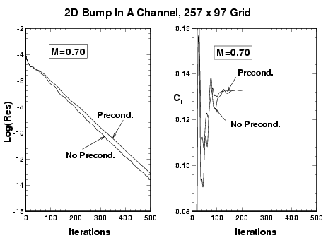
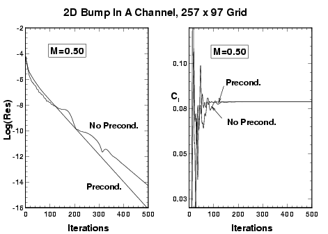
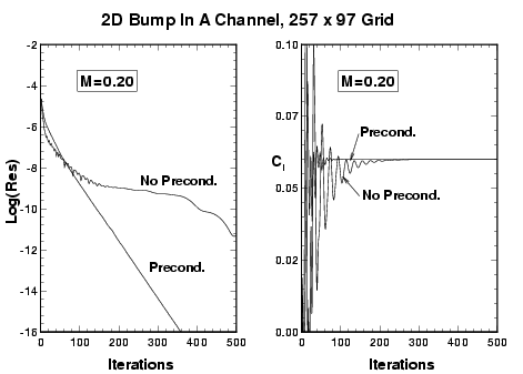
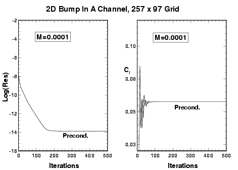
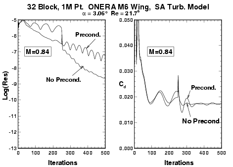
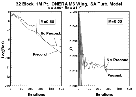
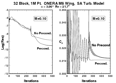
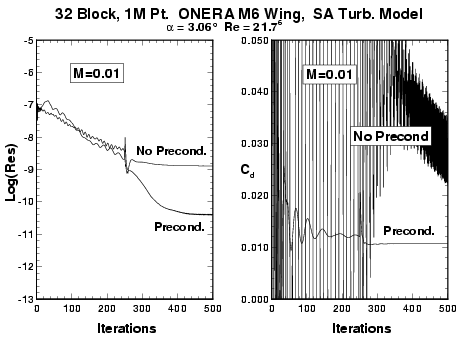
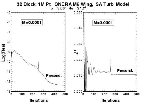
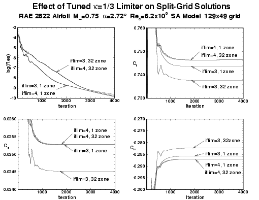
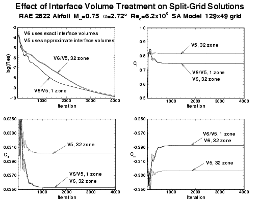
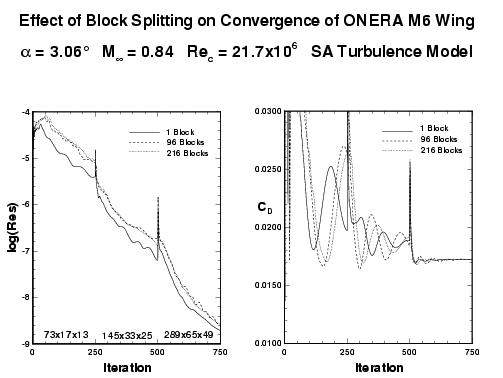
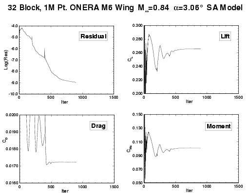
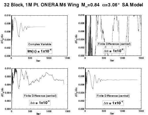
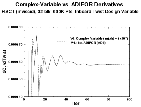
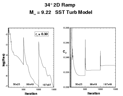
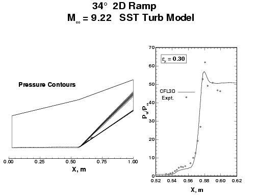
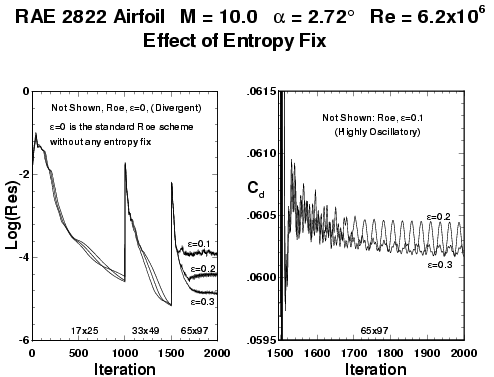
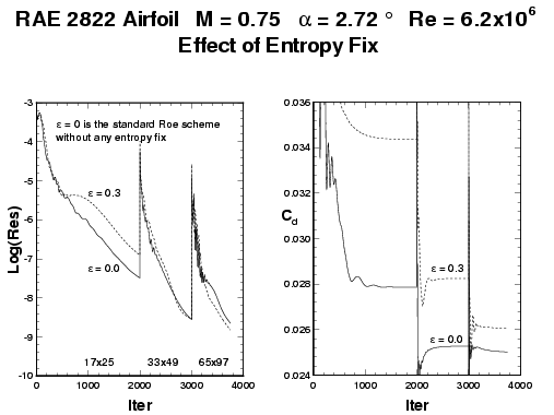
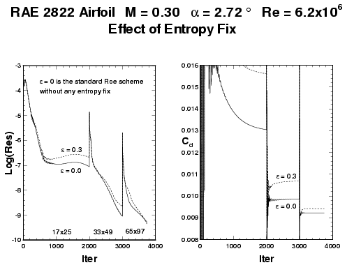